Cartoon of a STM32 connected to a PC with a timer in the background. — In this post, we’ll take the STM32 FFT algorithm from my blog “Writing Your Own FFT in Python and STM32” (link below) and focus on improving its execution speed. The goal is to minimize the number of clock cycles required to perform the FFT. To achieve this, we’ll remove unnecessary calculations, precompute the bit-reversal lookup table, enable compiler optimizations, activate the cache, and place buffers in faster memory. We’ll evaluate how each of these changes impacts performance, and compare our optimized algorithm to the CMSIS DSP library’s FFT.

Additional Resources:

We are going to implement this FFT in C on an STM32H723 (NUCLEO-H723ZG) using STM32CubeIDE and the HAL libraries. These steps should be similar for most other STM32 microcontrollers, though there may be small differences depending on the specific device or peripheral configuration.

As mentioned above this blog will be on optimizing the FFT code that we wrote in my Writing Your Own FFT in Python and STM32 blog.

We will “benchmark” how fast our FFT algorithm is running by counting the number of MCU clock cycles it takes to complete. In our case, we will be measuring from the time the DMA has filled (or half filled) the buffer with ADC values until the FFT has completed.

You can see my post on DWT + ITM + SWO and MCU Cycle Counting for how to set this up MCU cycle counting.

We will improve our FFT algorithm by doing the following:

Do not convert the ADC value to a voltage for all samples.
Use a look-up table for bit reversal.
Turn on compiler optimization.
Turn on cache and place data in faster DTCM RAM.
Convert our decimation-in-time (DIT) to a decimation-in-frequency FFT.

Lastly we will compare our algorithm to the CMSIS DSP library to see how well we did.

Some potential improvements that we are not exploring:

Using a Radix-4 or Radix-8 algorithm - we are just going to us Radix-2.
Using fixed-point - we are going to use floating-point.
Writing our own assembly code - we will just rely on the compiler to optimize as best as possible.

Baseline FFT

As mentioned above we will use the FFT algorithm as described in the Writing Your Own FFT in Python and STM32 blog. This FFT algorithm is a pretty basic implementation of a Radix-2 FFT and there is no attention to optimization other than pre-computing the twiddle factors into a look-up table (which does help the algorithm speed). With this we get our baseline speed:

Baseline = 832238 Cycles

Do Not Convert ADC Value to Voltage

The first low hanging fruit in our quest to optimize our FFT for speed is to remove unnecessary calculations. Converting each ADC value to its corresponding voltage is a waist of processing time. Converting the ADC value to a voltage is merely a scaling operation. The FFT does not care that it is an ADC value or voltage. We can simply send the ADC values into the FFT and then only convert the FFT outputs that we care about later (often you probably don’t care about the exact value). We will still convert the uint16 ADC value to a float.

Originally this occurs in both the HAL_ADC_ConvHalfCpltCallback( ) and the HAL_ADC_ConvCpltCallback( ). So as an example the HAL_ADC_ConvCpltCallback( ) function now looks like:

void HAL_ADC_ConvCpltCallback(ADC_HandleTypeDef *hadc) {

	dwtStartTime = DWT->CYCCNT;

	if (hadc->Instance == ADC1) {

		// Define a pointer to point at the middle of the adcBufer array
		uint16_t *p_adcBuffer = &adcBuffer_16b[FFT_SIZE];

		// Move data from adcBuffer to new fftAdc buffer for processing:
		// 		Bit-reveral re-arrage of data
		for (uint16_t i = 0; i < FFT_SIZE; i++) {
		
			// !!!!!!!!!!!!!!! Perform unint16 to float calculation later !!!!!!!!!!!!!!!!!!
			// fftAdc[2 * i] = adc16_to_voltage(*(p_adcBuffer + bit_reverse16(i, FFT_BITS))); // (-----Old Code------)
			
			fftAdc[2 * i] = (float)*(p_adcBuffer + bit_reverse16(i, FFT_BITS)); // Real part // (----New Code----)

			fftAdc[2 * i + 1] = 0.0f; // Imaginary part

		}

		// Flag that data is ready for FFT
		fftADC_ready = 1;
	}
}

And then we will wait until we need to convert an outputted FFT value. For example in the printFFT_Magnitude_MaxPossitive( ) function we output the frequency and magnitude of the peak frequency bin:

void printFFT_Magnitude_MaxPossitive() {

	float max = 0;
	uint16_t pos = 0;

	// Cycle through fftAdc array where even index is real, odd index is imaginary
	for (uint16_t i = 2; i < FFT_SIZE; i += 2) {

		// The k-th bin of the FFT
		uint16_t k = i / 2;

		// Calculate magnitude of bin data
		float magnitude = sqrtf(fftAdc[i] * fftAdc[i] + fftAdc[i + 1] * fftAdc[i + 1]);

		if (magnitude > max) {
			max = magnitude;
			pos = k;
		}

	}

	// Calculate corresponding bin frequency
	float fk = ((float) pos * 7500.0f) / (float) FFT_SIZE;

	// Print frequency and magnitude to serial
	char buffer[32];
      // snprintf(buffer, sizeof(buffer), "%.2f\t%.2f\n", fk, max); // (---Old Code----)
	snprintf(buffer, sizeof(buffer), "%.2f\t%.2f\n", fk, adc16_to_voltage(max)); // (---New Code----)
	HAL_UART_Transmit(&huart3, (uint8_t*) buffer, strlen(buffer), HAL_MAX_DELAY);

}

After this change we get the following improvement:

No ADC Convert to Voltage = 818859

Which is a 1.6% improvement from the baseline number of MCU cycles. Not huge but somewhat significant for such a small tweak.

Bit-Reversal Lookup Table

The next low hanging fruit is to change from calculating our bit-reversal “in the moment” to a simple lookup table (calculated at startup). In the later optimization attempts we will change from decimation in time FFT to a decimation in frequency FFT, which means that we would only perform bit-reversal at the end and specifically only for frequency bins of interest (a computational savings). Nonetheless, in our fft_512samp_init( ) function where we already precompute the twiddle factors we will add some code to also precompute our bit-reversal lookup table.

void fft_512samp_init() {

	// Create bit reversal lookup table
	for (uint16_t i = 0; i < FFT_SIZE; i++) {
		bitrev_table[i] = bit_reverse16(i, FFT_BITS);
	}

	// Zero out buffer (not needed but can be useful for debugging)
	for (int i = 0; i < 2 * FFT_SIZE; i++) {
		adcBuffer_16b[i] = 0;
		fftAdc[i] = 0;
	}

	// Pre-compute twiddle factors and interleave real and imaginary numbers in same array
	//		even indexes: real , odd indexes: imaginary
	for (uint16_t k = 0; k < FFT_SIZE / 2; k++) {
		float angle = 2.0f * PI * k / FFT_SIZE; // Calculate angle
		twiddle[2 * k] = cosf(angle); // Real
		twiddle[2 * k + 1] = -1 * sinf(angle); // Imaginary
	}

}

We will also modify HAL_ADC_ConvHalfCpltCallback( ) and HAL_ADC_ConvCpltCallback( ) to use the lookup tables:

void HAL_ADC_ConvCpltCallback(ADC_HandleTypeDef *hadc) {

	dwtStartTime = DWT->CYCCNT;

	if (hadc->Instance == ADC1) {

		// Define a pointer to point at the middle of the adcBufer array
		uint16_t *p_adcBuffer = &adcBuffer_16b[FFT_SIZE];

		// Move data from adcBuffer to new fftAdc buffer for processing:
		// 		Convert ADC values to float voltages
		// 		Bit-reveral re-arrage of data
		for (uint16_t i = 0; i < FFT_SIZE; i++) {

			// bit reversal lookup table
			fftAdc[2 * i] = (float)p_adcBuffer[bitrev_table[i]]; // Real part

			fftAdc[2 * i + 1] = 0.0f; // Imaginary part

		}

		// Flag that data is ready for FFT
		fftADC_ready = 1;
	}
}

After this change we get the following improvement:

Bit-Reversal Lookup Table = 766315

Which is a 6.4% improvement from the No ADC Covert to Voltage code. Which is somewhat significant. Overall we have a 7.9% improvement from our baseline.

Turn on O2 Optimization

Up to this point we are using no compiler optimization (O0). Now we are going to turn on compiler optimization, specifically O2 optimization.

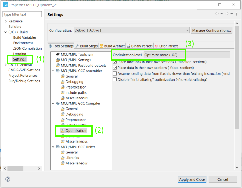
To enable this optimization we will open up out project properties dialog and navigate to C/C++ Build >> Settings and under the Tool Settings tab select MCU/CPU GCC Compiler >> Optimization and then set the optimization level to Optimized more (-O2).

Showing how to enable compiler optimization.

The only other change we’ll make at this point is to add the volatile keyword in front of our fftADC_ready variable. This tells the compiler not to optimize away reads or writes to this variable, since it may be modified outside the normal program flow — for example, by an interrupt handler or DMA complete callback. Without volatile, the compiler might assume the value doesn't change unexpectedly, which can lead to incorrect behavior during debugging or runtime.

volatile uint8_t fftADC_ready = 0;

With this relatively simple change we get the following improvement:

O2 Optimization = 152758

Which is a 80.1% improvement from the Bit-Reversal Lookup Table. Which is a huge improvement. Now we have a 81.6% improvement from our baseline.

( Should of really turned this on earlier … )

Using Cache

The STM32H7 has a built-in cache to make the MCU run faster by reducing the time it takes to access memory. It has two separate caches: one for instructions (I-cache) and one for data (D-cache). The instruction cache helps speed up code execution, while the data cache helps with fast access to variables and memory. We will use the data cache to speed up our FFT algorithm mainly by placing our FFT data in this faster cache memory. However we do need to be a little careful with how we work with cache memory. The data cache uses a write-back system, meaning changes to memory may stay in the cache for a while before being written back to the “normal” slower memory. Similarly the MCU wont necessarily read new data back into cache because it may not know that the original memory has changed. This can cause problems with peripherals like DMA, which access “normal” memory with out the MCU ’s knowledge. For example, suppose we have a Buffer A in normal memory which holds our ADC samples. The MCU smartly moves this data into cache and starts processing our FFT. Now we have a copy of Buffer A in our cache memory, and we still have our original Buffer A in normal memory. While the MCU is processing this data, our DMA fills Buffer A in the normal memory with new data. Eventually our program tells the MCU to start processing a new FFT, and the MCU starts processing the data in the cache. But in reality it is just re-processing the old data because it never went out to the normal memory to refresh. Unless you tell it to, it doesn’t know that it needs to get new data. It thinks that the data in the cache is the data you want to process. So developers need to tell the MCU to clean or invalidate the cache to keep things in sync or tell the MCU to never cache the memory in the first place.

In our FFT program, we currently use DMA to store ADC samples into a buffer called adcBuffer_16b, and then copy that data into another buffer called fftAdc. This second buffer uses floating-point format and stores real and imaginary parts in an interleaved layout, which is required for our FFT processing. The fftAdc buffer is then used directly in the FFT computation.

Once we enable the MCU cache, we need to be careful about memory regions that are shared between the MCU and peripherals like DMA. Specifically, we do not want the MCU to cache adcBuffer_16b, because the DMA writes to it independently of the MCU. If the MCU caches this region, it may read stale data that doesn't reflect the most recent ADC samples. To prevent this, we will configure the Memory Protection Unit (MPU) to mark the memory region used by adcBuffer_16b as non-cacheable. At the same time, we’ll allow the MCU to cache everything else to maximize performance.

Additionally, we’ll control where in memory our variables are stored. adcBuffer_16b will be placed in SRAM that is accessible by both the ADC and DMA. Meanwhile, performance-critical variables like fftAdc, the twiddle buffer, and the bitrev_table will be placed in DTCM (Tightly Coupled Memory), which offers much faster access for the MCU compared to regular SRAM.

In this section we’re not changing the FFT algorithm itself but rather optimizing where data lives in memory. In terms of speed hierarchy, cache is fastest, followed by DTCM, then SRAM.

With that understanding, let’s get started. First, we need to decide where in memory each buffer and variable will reside. Starting with adcBuffer_16b, we need to figure out:

Which bus ADC1 is connected to
Which DMA controller can transfer its data
Which SRAM region the DMA should write to

To answer the first question, open the STM32H723 reference manual and navigate to the Register Boundary Address table (Table 7, starting on page 134). This table shows which peripherals reside on which bus, and will help us identify how to route ADC1's data efficiently.

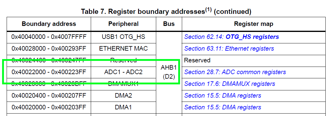
An exerpt from the STM32H723 reference manual showing which bus the ADC1 is connected to.

As we can see from the above image, the ADC1 is connected to the AHB1 bus. Now we will navigate to the System Architecture block diagram in order to find which DMA connects to AHB1 (Figure 1 on page 107):

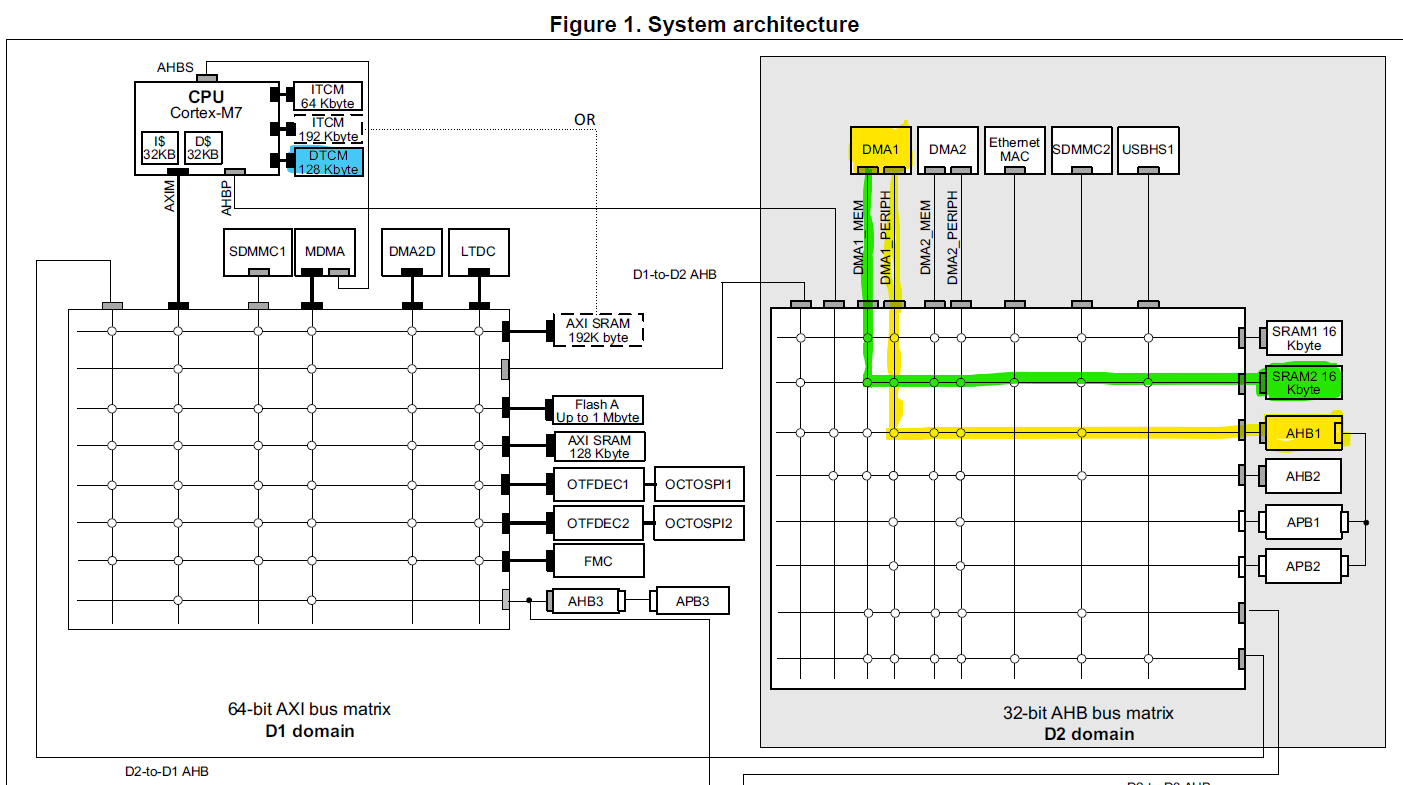
An exerpt from the STM32H723 reference manual showing the bus connection matrix.

In the System Architecture block diagram, I’ve highlighted the AHB1 bus in yellow, along with its path through the AHB bus matrix to DMA1. This shows how data flows from ADC1 to memory. In this configuration, DMA1_PERIPH retrieves samples from ADC1 via the AHB1 bus. From there, DMA1_MEM handles the transfer of these samples into SRAM2, which I’ve highlighted in green. (Alternatively, we could have chosen DMA2 or stored the samples in SRAM1, both are valid options depending on your memory layout.)

I’ve also highlighted the DTCM (Tightly Coupled Memory) region in the diagram. This is where we’ll place the rest of our buffers and variables such as the fftAdc array, the twiddle factor table, and the bit-reversal lookup table. Since DTCM is directly attached to the MCU core and bypasses the bus matrix, it provides much faster access compared to SRAM. That makes it ideal for performance-critical processing like FFTs.

Next, we need to do two things:

a) Tell the compiler where to place each variable in memory, and

b) Define those memory regions in the linker script so the linker knows where each section belongs.

Telling the compiler is straightforward as we just add a section attribute to the variable definition. For example, to place our twiddle factor lookup table in DTCM, we use the following:

__attribute__((section(".DTCMRAM"))) float twiddle[FFT_SIZE];

This tells the compiler to place the twiddle array into a custom section named .DTCMRAM.

We will also do this for the remaining variables:

// Buffer to store the samples from the 16-bit ADC
// Make adcBuffer twice the size as the number of samples we want for FFT
// Once the first half of the buffer fills, we process the first half while the second half
// starts filling up. And vice-versa.
volatile __attribute__((section(".SRAM2"))) uint16_t adcBuffer_16b[2 * FFT_SIZE];

// Array to store the converted voltage values from the 16-bit ADC samples
// FFT is of FFT_SIZE but this variable is twice the size to include real and imaginary values
// Where: even index = real, odd index = imaginary
__attribute__((section(".DTCMRAM"))) float fftAdc[2 * FFT_SIZE];

// Twiddle factors is FFT_SIZE/2 but is twice the size to include real and imaginary values
// Where: even index = real, odd index = imaginary
__attribute__((section(".DTCMRAM"))) float twiddle[FFT_SIZE];

// Bit reversal lookup table
__attribute__((section(".DTCMRAM"))) uint16_t bitrev_table[FFT_SIZE];

Now, we will modify the linker script to assign these section attributes to the appropriate memory region.

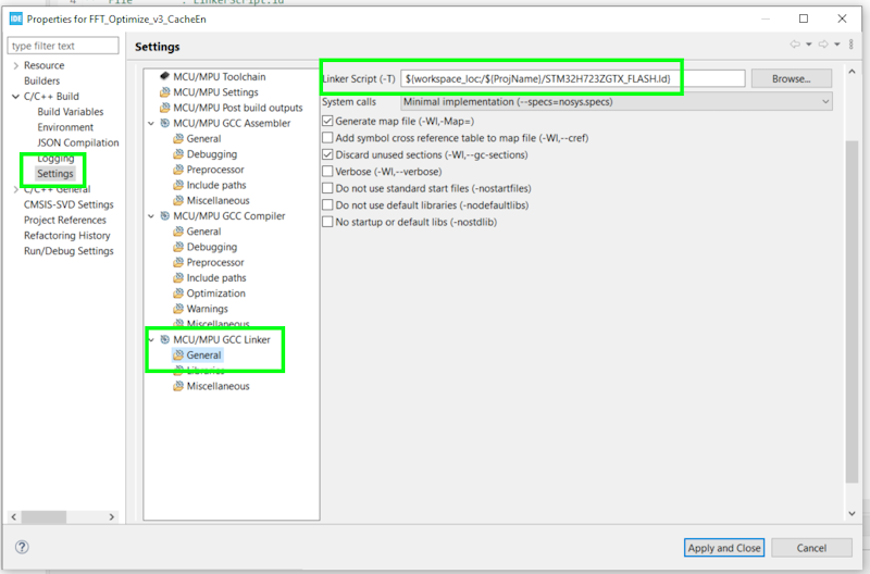
STM32CubeIDE by default will generate two linker scripts: STM32H723ZGTX_FLASH.ld and STM32H723ZGTX_RAM.ld . To figure out which script it is using, open the project properties and navigate to C/C++ Build >> MCU/CPU GCC Linker >> General and look at which linker script it is using as shown in the image below. In my case it is using the STM32H723ZGTX_FLASH.ld script.

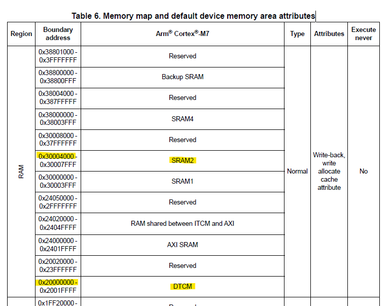
Image showing which linker script is being used in STM32CubeIDE.

Unfortunately I will not go through the linker script in any great detail. We will however add some additional lines of code to define our SRAM and DTCM memory. Note some of these regions may have already been specified in you linker scipt (ie. for me the DTCMRAM was already defined by default). Below shows an excerpt from the linker script with the added lines of code that we need for defining SRAM2 and DTCMRAM. Note that ORIGIN is the starting location of the DTCMRAM and SRAM2, and LENGTH is their region sizes. This information can be found in the Memory map and default device memory area attributes Table (Table 6 on page 132 of the STM32H723 reference manual).

/* Entry Point */
ENTRY(Reset_Handler)


... 


/* Specify the memory areas */
MEMORY
{
  ITCMRAM (xrw)    : ORIGIN = 0x00000000,   LENGTH = 64K
  DTCMRAM (xrw)    : ORIGIN = 0x20000000,   LENGTH = 128K
  FLASH    (rx)    : ORIGIN = 0x08000000,   LENGTH = 1024K
  RAM_D1  (xrw)    : ORIGIN = 0x24000000,   LENGTH = 320K
  SRAM2  (xrw)   : ORIGIN = 0x30004000, LENGTH = 16K
  RAM_D3  (xrw)    : ORIGIN = 0x38000000,   LENGTH = 16K
}

/* Define output sections */
SECTIONS
{

   ...
  
  
  .DTCMRAM :
  {
  	. = ALIGN(32);
    KEEP (*(.DTCMRAM))
    KEEP (*(.DTCMRAM*))
    . = ALIGN(32);
  } >DTCMRAM
	
  .SRAM2 :
  {
    . = ALIGN(4);
    KEEP (*(.SRAM2))
    KEEP (*(.SRAM2*))
    . = ALIGN(4);
  } >SRAM2 
	
  ...
}

An exerpt from the STM32H723 reference manual showing the base addresses of SRAM3 and DTCM ram.

Now that we’ve specified which memory regions the compiler should use for each variable, we can go ahead and enable the CPU cache to improve overall performance. However, enabling cache introduces a potential issue: since the DMA writes ADC samples directly to adcBuffer_16b, the CPU might read a stale (cached) version of that data unless we explicitly prevent caching for that region.

To solve this, we’ll also enable the Memory Protection Unit (MPU). The MPU allows us to mark specific memory regions, such as the one used for adcBuffer_16b, as non-cacheable. This ensures the CPU always reads the most up-to-date values written by the DMA, while still allowing the rest of the system to benefit from caching wherever it's safe and beneficial.

From within STM32CubeIDE we will open the .ioc file and in the Pinout & Configuration tool we will select the CORTEX_M7 settings, we can enable the CPU ICache and DCache as shown below.

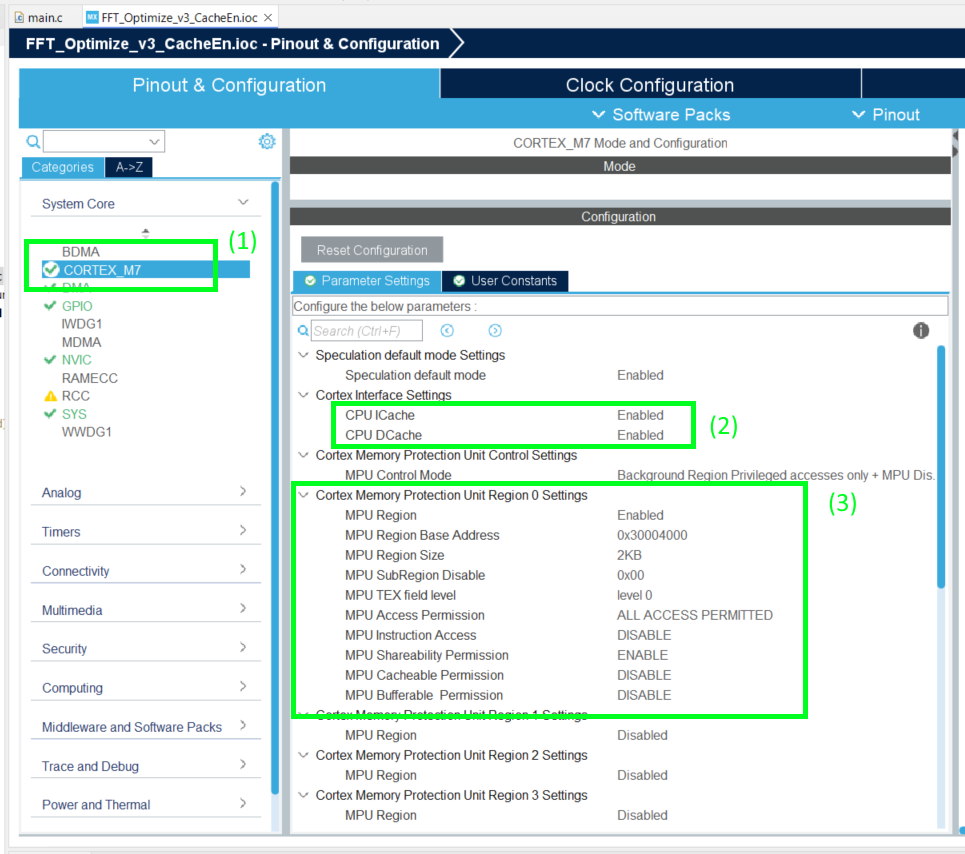
Image showing how to configure the cache and MPU in STM32CubeIDE's Pinout and Configuration tool.

Next, we’ll configure the Memory Protection Unit (MPU) by enabling one of its regions, in our case this is region 0. We’ll set the base address of this region to the start of SRAM2, which begins at address 0x30004000. The goal is to protect the memory used by the adcBuffer_16b variable from being cached by the CPU, since this buffer is continuously updated by the DMA.

The adcBuffer_16b buffer is 2 × FFT_SIZE, or 2 × 512 = 1024 bytes in total. MPU region sizes must be selected from a set of predefined powers-of-two, so we’ll round up and choose a region size of 2 KB, which is the next valid option above 1024 bytes.

Finally, we’ll disable the cacheable permission for this region. This tells the CPU not to cache any data in that region, ensuring it always reads fresh values directly from SRAM2.

With all these changes and settings in place we get the following improvement:

Cache = 56449

Which is a 63% improvement from the O2 Optimization. Which is also a huge improvement. Now we have a 93.2% improvement from our baseline.

Decimation-In-Frequency (DIF) FFT

In the previous sections we have improved our FFT by simply putting data in faster memory. In this section we will actually change our FFT algorithm from decimation-in-time (DIT) to decimation-in-frequency (DIF).

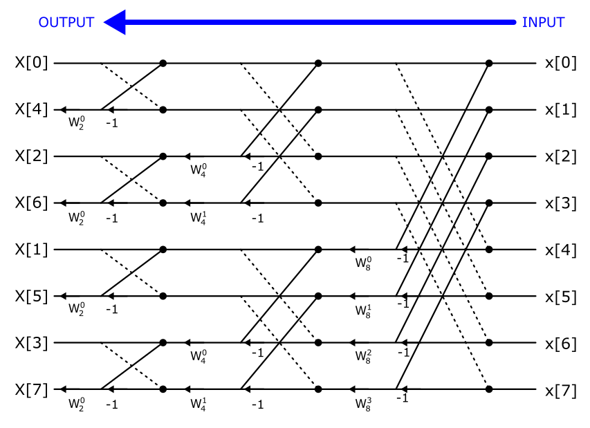
So as a reminder this is the butterfly diagram for the DIT:

A butterfly diagram of a 8 point DIT FFT.

The DIF butterfly swaps the input (x) and outputs (X) as well as change the direction of the arrows. As a result, the DIF implementation does not require bit-reversal at the beginning of the FFT process. If you need the entire frequency spectrum in order, you would then perform bit-reversal at the end. However, in many applications, you may only care about a specific portion of the FFT output around a known signal. In those cases, you can selectively perform bit-reversal only on the bins of interest, reducing the overall computation time.

A butterfly diagram of a 8 point DIF FFT.

Our DIF code is very similar to the DIT except:

DIT starts at stage 1 and works its way towards the last stage. Whereas the DIF starts at the last stage and works its way over to the first stage.
DIT butterfly multiplies the twiddle factor first, then add and subtract. Whereas the DIF will add and subtract, then multiply by twiddle factor.

void fft_dif_512samp() {

	// For each FFT stage
	for (uint16_t stage = FFT_BITS; stage >= 1; stage--) {

		// Butterfly size is 2^stage
		uint16_t m = 1 << stage;
		uint16_t mHalf = m >> 1;

		// At each FFT stage with group size m, you use the twiddle spacing FFT_SIZE/m
		uint16_t stride = FFT_SIZE / m;

		// For each frequency bin
		for (uint16_t k = 0; k < FFT_SIZE; k += m) {
			// For each corresponding butterfy
			for (uint16_t j = 0; j < mHalf; j++) {

				// Determine the index of first value in butterfly
				uint32_t i0 = k + j;

				//Determine the index of second value in butterfly
				uint32_t i1 = i0 + mHalf;

				// Determine index of required twiddle value for this butterfly
				uint32_t t_idx = j * stride;

				// Get real and imaginary parts of twiddle value
				float wr = twiddle[2 * t_idx];
				float wi = twiddle[2 * t_idx + 1];

				// Get real and imaginary parts of first value
				float xr = fftAdc[2 * i0];
				float xi = fftAdc[2 * i0 + 1];

				// Get real and imaginary parts of second value
				float yr = fftAdc[2 * i1];
				float yi = fftAdc[2 * i1 + 1];
   
				// Perform DIF butterfly
				// Bottom butterfly subtraction
				float tr = xr - yr;
				float ti = xi - yi;
                
				// Top butterfly addition
				fftAdc[2 * i0] = xr + yr;
				fftAdc[2 * i0 + 1] = xi + yi;

				// Twiddle multiply
				fftAdc[2 * i1] = wr * tr - wi * ti;
				fftAdc[2 * i1 + 1] = wr * ti + wi * tr;
			}
		}
	}
}

Then in our HAL_ADC_ConvHalfCpltCallback( ) function we no longer perform bit-reversal:

void HAL_ADC_ConvHalfCpltCallback(ADC_HandleTypeDef *hadc) {

	dwtStartTime = DWT->CYCCNT;

	if (hadc->Instance == ADC1) {

		// Normally commented out, but it can be useful to stop DMA for debugging
		// HAL_ADC_Stop_DMA(&hadc1);

		// Define a pointer to point at the begining of the adcBufer array
		volatile uint16_t *p_adcBuffer = &adcBuffer_16b[0];

		// Move data from adcBuffer to new fftAdc buffer for processing:
		// 		Convert ADC values to float voltages
		// 		Bit-reveral re-arrage of data
		for (uint16_t i = 0; i < FFT_SIZE; i++) {

			// !!!!! bit reversal lookup table
		    //fftAdc[2 * i] = (float)p_adcBuffer[bitrev_table[i]]; // Real part

			//!!!! No bit reversal, DIF
			fftAdc[2 * i] = (float) p_adcBuffer[i]; // Real part

			fftAdc[2 * i + 1] = 0.0f; // Imaginary part
		}

		// Flag that data is ready for FFT
		fftADC_ready = 1;
	}
}

Also adjust the HAL_ADC_ConvCpltCallback( ) function in the same way.

Finally we want to still find and print the maximum frequency and its bin value to our serial console using the printFFT_Magnitude_MaxPossitive( ) function. For the DIF FFT we will still search for the bin with the highest value (excluding the DC bin). However this time when we calculate the frequency we will perform the bit-reversal on the single frequency bin as opposed to the entire spectrum.

What we had when we were doing DIT:

float fk = ((float) pos * 7500.0f) / (float) FFT_SIZE;

For the DIF we now have to perform the bit-reversal:

fk = ((float) bitrev_table[pos] * 7500.0f) / (float) FFT_SIZE;

Thus our printFFT_Magnitude_MaxPossitive( ) function now looks like:

void printFFT_Magnitude_MaxPossitive() {

	float max = 0;
	uint16_t pos = 0;

	// Cycle through fftAdc array where even index is real, odd index is imaginary
	for (uint16_t i = 2; i < FFT_SIZE; i += 2) {

		// The k-th bin of the FFT
		uint16_t k = i / 2;

		// Calculate magnitude of bin data
		float magnitude = sqrtf(fftAdc[i] * fftAdc[i] + fftAdc[i + 1] * fftAdc[i + 1]);

		if (magnitude > max) {
			max = magnitude;
			pos = k;
		}
	}

	float fk = 0.0f;
	if (bitrev_table[pos] < FFT_SIZE / 2) {
		// Calculate corresponding bin frequency
		fk = ((float) bitrev_table[pos] * 7500.0f) / (float) FFT_SIZE;
	} else {
		// Calculate corresponding bin frequency (as negative value - but we change it to abs())
		fk = -1*((((float) bitrev_table[pos] - FFT_SIZE) * 7500.0f) / (float) FFT_SIZE);
	}

	// Print frequency and magnitude to serial
	char buffer[32];
	snprintf(buffer, sizeof(buffer), "%.2f\t%.2f\n", fk, adc16_to_voltage(max)); 
	HAL_UART_Transmit(&huart3, (uint8_t*) buffer, strlen(buffer), HAL_MAX_DELAY);
}

With all these changes and settings in place we get the following improvement:

DIF = 56449

Which is a 11% improvement from the Cache. Now we have a 94% improvement from our baseline which is slightly better than before.

So this is all the improvements we will attempt in this blog. In the next section we will compare our FFT algorithm with the CMSIS-DSP’s FFT algorithm to see how well we have done.

CMSIS-DSP’s FFT Comparison

As mentioned above, the purpose of this section is to compare our FFT algorithm to CMSIS-DSP’s FFT algorithm. More specifically, we are comparing to their complex FFT with 32bit floating point called CFFT F32. This is not a fair comparison as their algorithm supports Radix-8 and Radix-4 butterflies whereas ours is only Radix-2. Simply going from Radix-2 to Radix-4 would give you about 25% improvement alone.

The information on the CMSIS-DSP library and Github repo can be found here.

Setting it up was a bit of a pain for me. I assume there is a far better way of doing it but I will walk you through what I did.

1. Download the CMSIS-DSP library

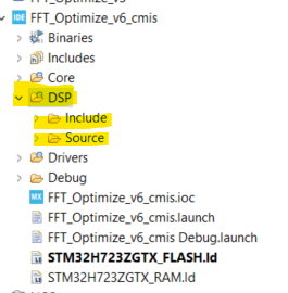
2. Create a new source folder in STM32 (I called it DSP) and within that folder create a Include and a Source folder:

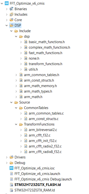
Image showing the folder setup for the CMSIS-DSP library.

3. Include the files and sub-folders as shown in the image below. I “figured out” which files were needed for the most part this was done with some trial and error. I knew that I needed the arm_cfft_f32.c and the arm_math.h files but I didn’t quite know what other files were needed. You can read the .h and .c files to figure out what is needed but sometimes it is just easier to let the compiler tell you what is missing and then you add the files until the errors go away (I know real amature stuff).

Image showing all the required .h and .c files to run the cfft F32 FFT from CMSIS-DSP.

Now that we have all our files inside our project, we will go to our main.c file and we will include the arm_math.h file and define which ARM core we are using:

#define ARM_MATH_CM7
#include "arm_math.h"

We will also add a cfftHandler to hold basic information that the CMSIS cfft algorithm will use:

arm_cfft_instance_f32 cfftHandle;

Next in our main(void) function we will comment out our FFT initialization function fft_512samp_init() and add CMSIS’s initialization:

int main(void) {

	...

	// Initialize FFT (mainly calculate twiddle factors)
	//	fft_512samp_init();

	arm_cfft_init_512_f32(&cfftHandle);

	// Start ADC with DMA
	if (HAL_ADC_Start_DMA(&hadc1, (uint32_t*) adcBuffer_16b, 2 * FFT_SIZE) != HAL_OK) {
		Error_Handler();
	}

	while (1) {
	
	...
	
	}
}

Inside out main while(1) infinite loop we will comment out our FFT function fft_dif_512samp() and add CMSIS’s arm_cfft_f32( ) function:

while (1) {

	// If ADC has completed filling buffer + We moved data to fftAdc (which is bit reversed
	// and converted to a float voltage value)
	if (fftADC_ready) {

		// Perform decimation in time FFT
		//	fft_dif_512samp();

		arm_cfft_f32(&cfftHandle, fftAdc, 0, 1);

		dwtEndTime = DWT->CYCCNT;
		dwtTotalTime = dwtEndTime - dwtStartTime;
		printf("%lu\n", dwtTotalTime);

		//Print all the FFT data as magnitude
		printFFT_Magnitude_MaxPossitive();

		// Reset ready flag
		fftADC_ready = 0;
	}

	/* USER CODE END WHILE */

	/* USER CODE BEGIN 3 */
}

The function CMSIS cFFT function has the following form:

arm_cfft_f32( pointerHandler, pointerData, fft_or_iff, bitReversal )

Where pointerHandler is a pointer to our cfftHandle which was initialized earlier,

pointerData is a pointer to our sample data inside the fftAdc buffer,

fft_or_iff is a flag that tell the function to perform a FFT or a IFFT. If set to 0: FFT, set to 1: IFFT

bitReversal is a flag that tells the function to perform bit-reversal of output data. If set to 0: no bit-reversal, set to 1: perform bit-reversal.

And that is pretty much all you need to do. With all these changes and settings in place we get the following improvement:

CMSIS = 37339

Which is a 25% improvement from the DIF. Now we have a 96% improvement from our baseline.

Conclusion

We saw significant speed improvement from simply turning on compiler optimization and using the MCU cache. The other tweaks we made certainly improved our code. The optimized CMSIS-DSP performed better than our simple algorithm. However I think our Radix-2 FFT algorithm did okay given that the CMSIS algorithm is using a more efficient Radix-8 algorithm (technically it would of been a combination of Radix-8 and Radix-2 due to us using 512 samples).

Optimizing Custom FFT’s Speed on STM32