Numerically Controlled Oscillator in Python and STM32

In this post, I’ll cover the basics of creating a Numerically Controlled Oscillator (NCO) from the ground up. An NCO is a digital signal generator that uses a phase accumulator and a waveform lookup table to produce precise, periodic signals—usually sine, square, or triangle waves. These waveforms are generated entirely in the digital domain, making NCOs extremely useful in systems where analog components are limited or where digital precision is required.
NCOs are widely used in a variety of applications, including digital communications, frequency synthesis, software-defined radio (SDR), and audio signal generation. Their ability to generate stable, tunable frequencies with minimal hardware makes them a valuable tool in embedded and signal processing systems.
We’ll begin by modeling the NCO in Python. This lets us explore and visualize the underlying concepts like phase resolution, tuning words, and waveform table indexing without worrying about hardware limitations. Once the behavior is well understood, we’ll transition to implementing the NCO in C on an STM32 microcontroller, where we’ll focus on efficient fixed-point arithmetic and real-time constraints.
Additional Resources:
Numerically Controlled Oscillator Overview
In its simplest form, a Numerically Controlled Oscillator (NCO) consists of four main blocks:
Phase Accumulator (PA) - This block adds a fixed value (known as the frequency control word) to its previous value on every clock cycle. It effectively generates a ramp signal that represents phase over time.
Phase Truncation - While not strictly required, this block is used to reduce the number of bits from the phase accumulator before feeding it into the next stage. This helps reduce the memory needed for the lookup table used in the next block. Also known as a phase quantizer.
Phase-to-Amplitude Converter (PAC) - This block converts the truncated phase value into an amplitude value. It typically uses a lookup table (LUT) that maps the truncated phase values to waveform amplitudes.
Digital-to-Analog Converter (DAC) - The final block converts the digital amplitude value into an analog signal, usually a voltage. This output represents the generated waveform.
A block diagram of this basic NCO structure is shown below.

The phase accumulator consists of a delay block (often represented as Z−1) and a summing block. The two inputs to the summing block are the frequency control word (FCW) and the previous output of the accumulator. As the name suggests, the frequency control word determines the frequency of the NCO output.
On each clock cycle, the frequency control word is added to the accumulator's previous value, causing the phase to increment steadily over time. This creates a sawtooth-like phase ramp, which drives the waveform generation process.
The output frequency of the NCO is given by:

where FCW is the value of the frequency control word, Fclk is the frequency of the clock, and N is the number of bits in the accumulator. In our example, we will use
FCW = 1638
Fclk = 10kHz
N = 16
Thus Fout = 250Hz
The frequency control word is typically one bit less than the width of the phase accumulator, N–1 bits. This is because the maximum output frequency of an NCO is limited by the Nyquist Theorem, which states that the highest representable frequency is half the clock frequency, or Fclk/2. In a binary system with base 2, this is one bit less:
2^15 = 32768
2^16 = 65536
2^16 / 2 = 65536 / 2 = 32768 = 2^15
The phase-to-amplitude converter in this NCO is implemented as a simple lookup table that takes a phase value as input and outputs a 12-bit value to drive the digital-to-analog converter. The lookup table could contain values that would create either a sine wave, square wave, saw wave, triangle wave, or some other special arbitrary waveform. Without a phase truncation block, the lookup table would need to cover the entire range of the accumulator. For example, with a 16-bit accumulator, the table would require 2^16 = 65,536216 = 65,536 entries, or approximately 64 KiB of memory. If we used a 32-bit accumulator, the table size would explode to 2^32 entries or 4 GiB, which is clearly impractical for most embedded systems.
To reduce memory usage, we introduce a phase truncation block. Instead of using the entire accumulator output, we use only the most significant bits to index the lookup table. In this example, we’ll use the top 8 bits of the accumulator, resulting in a lookup table with 2^8 = 256 entries. This drastically reduces memory requirements to just 256 bytes, while still preserving the basic shape and periodicity of the waveform. I would note that this is a pretty small lookup table and you may want to use a larger one in your application.
The digital-to-analog converter simply converts the output of the phase-to-amplitude converter into a corresponding analog voltage.
Implementing NCO Using Python
Before starting I am using Python 3.13 along with the following libraries:
Numpy for array handling, math, and plotting
Matplotlib for plotting
For my IDE, I’m using Spyder, since its layout is very similar to Matlab, which makes it great for this. To see how I setup my workspace see Using Spyder with Python Virtual Environment.
Lets start by importing our required libraries for this tutorial:
import numpy as np
import matplotlib.pyplot as plt
Next we will create a Python generator to emulate the clock driving the phase accumulator. For more information on Python generators see Programiz’s Python Generators tutorial.
In short, the function clockNCO(frequency, captureTime) takes the clock frequency and desired capture time as inputs. When used as an iterable, it yields the time of each clock cycle, one per cycle, based on the specified frequency.
# A generator that will simulate a system clock for the NCO
# frequency = the frequency of the clock
# captureTime = the amount of time we want to run the simulation of the NCO
def clockNCO(frequency, captureTime):

    # Calculate the clock period
    period = 1/frequency

    # For each clock cycle in the capture time
    for trigger in range(int(captureTime/period)):
        yield (trigger * period) # Return the current time
Now lets start defining our variables:
frequencyControlWord - Our frequency control word (needs to be less than 2^15)
accumulator - The 16bit phase accumulator
trunked - A variable used to hold the result after the phase truncation
sinWaveLUT - The phase-to-amplitude converter’s lookup table of a sine wave.
dacOutput - A python list which will fill with the DAC output values
dacTime - A python list which will fill with time corresponding the the DAC output values
# Define our frequency control word
frequencyControlWord = 1638

# Define our accumulator and phase truncation size and initial values
accumulator = np.uint16(0)
trunked = np.uint8(0)

# Create out lookup table for the PAC
# Note for this example we will have the lookup table loaded with
# the voltages that the DAC would output
sinWaveLUT = np.sin(np.linspace(0, 2*np.pi, 256))

# Define lists/arrays that will keep track of the DAC output over time
dacOutput = []
dacTime = []
Note: In the block diagram of the NCO, the phase-to-amplitude converter’s lookup table should contain 12bit digital values for the DAC. In this simulation we are going to instead have the actual DAC “analog” values inside the lookup table.
Now we get to the actual NCO implementation. We start our code with a loop that uses the clock generator. Inside this loop, we separate the operations into two categories: those that happen on the clock edge, and those that happen immediately afterward. The operations that occur right on the clock edge include phase truncation, the phase-to-amplitude conversion, and the DAC output. These are all synchronous steps that operate based on the current state of the system. After these, we update the phase accumulator by adding the frequency control word. This update happens after the clocked operations are complete.
# For each item in the clock NCO generator, simulate the DAC output of the NCO
# We are running a 10kHz clock for 10ms.
for trigger in clockNCO(10e3, 10e-3):

    # Syncronous Operations *************************

    # Perform phase truncation by shifting the 8 MSB down to LSB
    trunked = accumulator >> 8

    # The DAC output equals the lookup table value
    dacOutput.append( sinWaveLUT[trunked] ) # DAC value/voltage
    dacTime.append(trigger) # DAC time

    # Asyncronous Operations *************************

    # Increment the accumulator
    # Note because accumulator is np.uint16(), when accumulator > 2^16
    # Python will roll-over the accumulator value like it would in an
    # embedded system. Note you may get a Python warning.
    accumulator += frequencyControlWord


# Plot the simulated NCO
plt.figure()
plt.plot(dacTime, dacOutput)
plt.title("NCO Output")
plt.xlabel("Time (s)")
plt.ylabel("Voltage (V)")

Below is the complete code.
Implementing NCO on STM32 with C
For the next part, we are going to implement this NCO on an STM32H723 (NUCLEO-H723ZG) using STM32CubeIDE and the HAL libraries. These steps should be similar for most other STM32 microcontrollers, though there may be small differences depending on the specific device or peripheral configuration.
First step is creating a new STM32 project, selecting the microcontroller, give it a name, and use C as the targeted language.
If it is not already opened by default, double click the .ioc file from the project explorer to use the STM32CubeIDE configuration tool. The next steps will take place in the Pinout and Configuration tool provided by STM32CubeIDE:
For debugging we will select PA14 and PA13 as SWCLK and SWDIO respectively. To configure these we will go to the Trace and Debug category >> Debug >> Serial Wire

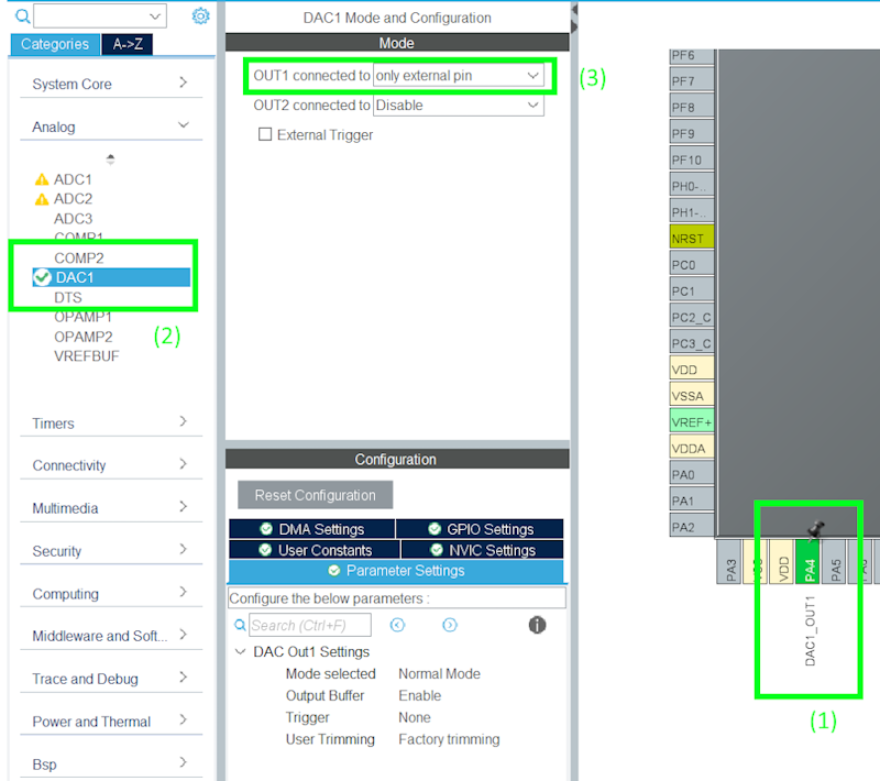
Next we will configure the digital-to-analog converter (DAC) on pin PA4 as DAC1_OUT1. To configure the DAC, we will go to the Analog category >> DAC1 >> Set OUT1 connected to only external pin.
Lastly we will configure the timer used as the phase accumulator clock. For this we will use TIM1 which will be generated by the internal clock.
Before configuring TIM1, we are going to want to check what frequency it is running at. But before we can do that we need to find which bus TIM1 belongs to.
From the STM32H7 reference manual, we navigate to the Memory and Bus Architecture section and we find the Register boundary addresses table. In the peripheral column we then find the TIM1 which exists on the APB2 bus (page 137).

Now that we know which bus the TIM1 belongs to, let check its clock frequency. From the STM32CubeIDE configuration tool (.ioc) navigate to the Clock Configuration tab and find the APB2 Timer Clocks.
As we can see in the image below the APB2 timer clocks are running at 96MHz - thus TIM1 internal clock is 96MHz.

For this example we are going to use a fairly slow clock speed for the phase accumulator of 10kHz. We need to configure TIM1’s 96MHz frequency to 10kHz using both the prescaler and the counter period.
First we will use the prescaler to scale the TIM1 frequency to 1MHz:

Next we will set the counter period of the timer to give us our 10kHz phase accumulator clock:

Thus from the above calculations we want to set the prescaler = 96 and the counter period = 100.
Since both the prescaler and counter period is always at least 1 (ie cannot be 0) we will enter the prescaler = 96-1 and counter period = 100 -1
To configure TIM1, we will go to the Timers category >> TIM1:
Clock Source = Internal Clock
Prescaler = 96-1
Counter Period = 100-1

The last thing we want to do is enable interrupts for TIM1 by going into the NVIC Settings tab and selecting TIM1 update interrupt.

That should be all of the configurations we need to do. To generate the code go to Project >> Generate Code.
Now working in the main.c file lets first add our sine wave lookup table between the /* USER CODE BEGIN PV */ and /* USER CODE END PV */ comments:
Where the { … } holds the values for the sine wave. The easiest way to generate these values is to use Python as follows:
Where sinWaveLUT will have the 12bit DAC values corresponding to a sine wave. We will now update the sineLUT[256] with the generated values:
Still within the /* USER CODE BEGIN PV */ and /* USER CODE END PV */ comments, lets define the frequency control word and accumulator unsigned 16bit variables.
Next we will go into the int main(void) {} function of our main.c file and within the /* USER CODE BEGIN 2 */ and /* USER CODE END 2 */ comments we will start the DAC and the TIM1 with interrupts enabled.
Lastly, we want to add a callback for the TIM1 interrupt so that code is executed each time TIM1 completes its timer period. Within the /* USER CODE BEGIN 4 */ and /* USER CODE END 4 */ comments near the end of the main.c file, we will add the callback void HAL_TIM_PeriodElapsedCallback(TIM_HandleTypeDef *htim) . Within this function we will add a check to see if TIM1 called the interrupt followed by the NCO code.
Just like we did in the Python code, we'll begin with the operations that occur on the clock edge, followed by those that happen shortly after. First, we perform phase truncation on the phase accumulator value. Then we set the DAC output voltage. Finally, we increment the phase accumulator by the frequency control word to prepare for the next cycle. Note that when the phase accumulator value exceeds 2^16, it wraps around to zero. This behavior is expected and reflects the natural overflow of a fixed-width 16-bit register.
If you want to see the complete code for this NCO, check out on Github
Now that this is complete we can run this code on the STM32. Connecting an oscilloscope attached to pin PA4 (DAC output) and we get the following waveform.
Notice that we do not get as nice of a sine wave as predicted in the python script. This is due to the fact that the python model does not account for the sample-and-hold of the DAC output which gives us this staircase look.

One way we can reduce this is by increasing the frequency of the phase accumulator from 10kHz to 100kHz. We can easily change this by changing TIM1’s counter period = 10-1 and then changing the frequency control word to 164 to maintain the same frequency of the output sine wave.

The other ways to do this is to increase the size of the phase-to-amplitude lookup table and increase the the number of bit of the phase accumulator.