Using Spyder with Python Virtual Environment

In this post, I’ll walk you through how I set up my Spyder IDE to use a Python virtual environment and enable interactive plots with ipympl.

Note I am using Spyder 5.5.1, Python 3.13, and Windows for this tutorial.

Spyder is a great IDE for scientific and engineering applications in Python - especially if you're coming from a Matlab background. Its interface closely resembles Matlab, making it easier to work with arrays, matrices, and plots compared to something like Visual Studio Code. This is particularly helpful when analyzing data during debugging or after your code runs.

It also features an easily accessible IPython console, which is super convenient when you want to test things out in “real time.”

Bottom line: If you like Matlab, you’ll probably enjoy using Spyder for Python.

I can confirm that this setup does work with Spyder 6 !

In addition to using Spyder, I also want to enable interactive plots with ipympl and work within a virtual environment. Interactive plots make it easy to zoom into your data, rename axes and titles, and use your cursor to inspect specific data points. For this, I’ll be using ipympl, which works well for this. One catch with Spyder is that, as far as I know, interactive plots only work when they appear in a separate window, which requires a bit of extra setup.

A virtual environment in Python is like a separate box where you keep all the tools and libraries your project needs. Without one, everything gets installed in the same place, and that can lead to problems - like running into errors if two projects need different versions of the same library. Using a virtual environment keeps things organized and helps make sure your code works the same way every time, even if you come back to it later or share it with someone else.

Creating the Virtual Environment

To start this tutorial I am going to assume that you have Spyder and Python installed.

Step 1 - Create a folder for your virtual environment

Lets create a folder where we want our virtual environment to exist. Usually I also use this folder as like a project folder and all the python scripts in that folder use that virtual environment. Then I am going to open the terminal / command prompt / powershell and navigate it to your new folder using:

cd folderLocation

Where folderLocation is the location of your new folder. In my case this is at .\Documents\Python\Demo\demoVenv and it would look something like:

cd .\Documents\Python\Demo\demoVenv

Step 2 - Create your virtual environment

We will create the virtual environment inside this folder by typing the following into the terminal:

python -m venv venvName

Where venvName is the name of the virtual environment. In my case I will call it myVenv and it would look like:

python -m venv myVenv

After a couple seconds your virtual environment should be created and you will notice a new folder with the name of your virtual environment in your folder.

Setting Up the Virtual Environment

Now we have a brand new virtual environment, but there aren’t any libraries installed in it yet. Since I am going to be using this enviroment for digital signal processing, I am going to want to install the following libraries:

• Numpy for array handling, math, and plotting

• Scipy for more advanced signal processing and statistics

• Matplotlib for plotting + ipympl for interactive plots

• PyQt5 which is needed to have our interactive plots appear in a separate window. In general this library is used for graphical user interfaces (GUI) but we are only using it to support for interactive plots.

• Spyder-kernels a library that allows the Spyder IDE to run code in a separate Python process (kernel), enabling features like the IPython console and variable explorer to work properly.

Many other libraries will also be installed along with these, as they are required dependencies.

Before we start installing any libraries, we need to activate our virtual environment - otherwise, the libraries will be installed in the global Python environment.

Step 3 - Activating your virtual environment

As mentioned, we need to activate the newly created virtual environment before installing any libraries to it. Note this is the same steps for activating the virtual environment if you want to install a different library not mentioned in this tutorial at a later time. Within the new folders that were created when we created our virtual environment there is an activate script that we are going to run.

In our terminal we should still be in the folder from Step 1 with our virtual environment. To activate our virtual environment use the following command:

.\venvName\Scripts\activate

Where venvName is the name of the virtual environment. In my case I will call it myVenv and it would look like:

.\myVenv\Scripts\activate

Once completed the next time in the terminal should have the prefix (venvName) as shown below.

Step 4 - Installing libraries

As mentioned above we are going to install numpy, scipy, matplotlib, ipympl, PyQt5, and spyder-kernels.

Enter in the following commands one at a time:

pip install numpy
pip install scipy
pip install matplotlib
pip install ipympl
pip install pyqt5

Some Notes:

• You do not need to install scipy (ie. you can skip that command). You need all the other ones.

• We have not installed the spyder-kernels yet because I suspect this is going to depend on the version of Spyder that you are running with. As we will see later, Spyder will tell you exactly which version of spyder-kernels to install so do not close your terminal just yet.

• If you want to see a list of everything you have installed use the command:
  
  pip list
  

• If you want to uninstall one of your libraries use the command:
  
  pip uninstall library
  
  Where library is the name of the library you want to uninstall

• If you want to save a list of all your installed libraries to make future setups faster, use the following command:
  
  pip freeze > requirements.txt
  
  Then when you want to install all of the libraries listed in requirements.txt, use the command:
  
  pip install -r requirements.txt

Setting Up Spyder

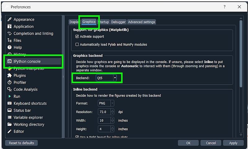
Step 5 - Configure Spyder’s graphics backend / plots

By default Spyder will create plots inside of it’s plot panel, which can be nice. The downside is that these plots are not interactive. So in this step we want to configure Spyder to create plots using PyQt5 which will then be interactive. With Spyder running, go to Tools and then Preferences to open the Preferences window. In the left side panel, select IPython console and then select the Graphics from the tabs at the top. In the Graphics backend section, click on the drop down menu and select Qt5.

Step 6 - Configure Spyder’s Python interpreter

Again go to Tools and then Preferences to open the Preferences window. In the left side panel, select Python interpreter and then select the option button Use the following Python interpreter. Next either manually enter the location or click on the file button on the right side of the text box. Navigate to your virtual environment folder, then go into Scripts, then select python.exe. For example

… /demoVenv/myVenv/Scripts/python.exe

Is where the python.exe file is located in my virtual environment.

Step 7 - Install spyder-kernels

Now with these changes made, click Apply and OK them in the Preferences window.

Next go to Consoles and select Restart kernel.

From here you should see an error in the IPython console and the instructions for which spyder-kernels to install. Next go back to your terminal (make sure you still have your virtual environment activated) and copy and paste the pip command that Spyder gives you. In my case this is:

pip install spyder-kernels==2.5.*

Restart your kernel again (might need to restart Spyder) and you should be good to go.

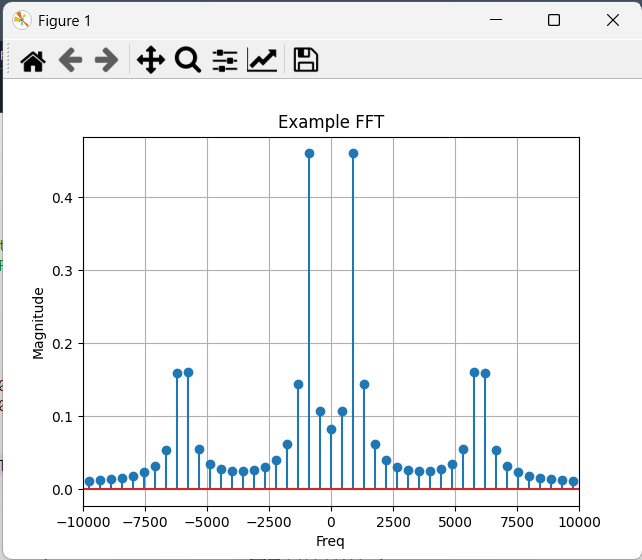
Try using the following code to plot the FFT of two sine waves.

import numpy as np
import scipy.signal as sig
from scipy.fft import fft, fftfreq
import matplotlib.pyplot as plt

# To improve our spectral leakage we can increase the number of sample points
# ie. increase our capture time
# Increasing sample rate does not do anything for us

# Number of sample points
N = int(5*225)

# Sample rate
Fs = 5*100e3
Ts = 1/Fs

print(f"Capture time: {N*Ts}s")
print(f"Capture Freq: {1/(N*Ts)}s")

# Signals
f1 = 1e3
f2 = 6e3

x = np.linspace(0.0,N*Ts, N, endpoint=False)
y = np.sin(f1*2.0*np.pi*x) + 0.5*np.sin(f2 * 2.0*np.pi*x)

yf = fft(y)
xf = fftfreq(N, Ts)

plt.figure()
plt.stem(xf, 1/N *np.abs(yf))
plt.grid()
plt.xlim(-10000,10000)
plt.ylim()
plt.show()