FFT with Python

In this post, I’ll walk through the basics of creating and plotting a discrete-time signal, then show how to analyze it in the frequency domain using the Fast Fourier Transform (FFT). Understanding how a signal behaves in both the time and frequency domains is a key skill in digital signal processing, and the FFT is one of the most powerful tools for doing that.
We’ll start by building a simple signal in Python, visualize it, and then compute its frequency spectrum. From there, we’ll run into a common and sometimes confusing issue called spectral leakage. It’s an important concept that affects how you interpret frequency-domain plots, especially when working with real-world signals.
To address spectral leakage, we’ll introduce windowing, a technique that tapers the edges of the signal before performing the FFT. We’ll explore a few popular window types, understand how they work, and see their effects through practical examples.
This post is meant to be hands-on and applied.
Additional Resources:
Before starting I am using Python 3.13 along with the following libraries:
Numpy for array handling, math, and plotting
Scipy for more advanced signal processing and statistics
Matplotlib for plotting
For my IDE, I’m using Spyder, since its layout is very similar to Matlab, which makes it great for this. To see how I setup my workspace see Using Spyder with Python Virtual Environment.
Lets start by importing our required libraries for this tutorial:
import numpy as np
import scipy.signal as sig
from scipy.fft import fft, fftfreq
import matplotlib.pyplot as plt
Creating a Signal
A continuous signal is one that exists for all points in time and can take on any value at any moment. Think of something like an analog voltage or sound wave in the air which are smooth and unbroken. However, when working with digital systems like computers or microcontrollers, we can’t handle infinitely detailed signals. Instead, we need to sample the signal at specific intervals, turning them into a discrete-time signal.
On top of that, we also can’t capture a signal forever - so we take only a limited time window of it (capture window). These two steps sampling in time and limiting the duration are necessary for processing signals in the digital world.
We will start by plotting a 1kHz sine wave but we will have a very high sample rate to “emulate” a continuous time sine wave. We will then decrease the sample rate to create a sine wave that no longer looks continuous as a comparison.
Lets defining our capture time as 5ms (ie. how long in time we will sample data for before analyzing it):
captureTime = 5e-3
Then we will define our very high sample rate of 10MHz:
Fs = 10e6
We can calculate the total number of samples by multiplying the capture time by the sample rate. It may be useful to print out the result just as a reference:
N = int(captureTime * Fs)
print(f"Number of Samples: {N}")
Okay now we are going to create an array of sample times using numpy’s linspace function which has the following syntax:
np.linspace( Start , End , NumberOfPoints )
Thus for our use case we will start at 0s, end at captureTime, and we will have N number of points (or samples):
x = np.linspace(0, captureTime, N, endpoint=False)
The last attribute “endpoint=False” tells linspace not to include the ending sample point. Thus our x array goes from 0 to 0.0049999s.
Now we will create our signal where f1 is the frequency of our sine wave:
f1 = 1e3
y = np.sin(2*np.pi*f1*x)
Putting this all together and plotting the waveform gives us the following:
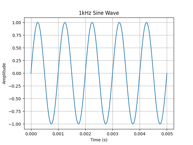
# How long of a signal in time we want to display/capture
captureTime = 5e-3

# Sample rate
Fs = 10e6

# Given the captureTime and the sample rate, this is the total number of samples
N = int(captureTime * Fs)
print(f"Number of Samples: {N}")

# Create an array of time samples from 0 to our captureTime and have N samples
x = np.linspace(0, captureTime, N, endpoint=False)

# Create our signal but sampled at points from our x array
# Our signal will be a 1kHz sinewave
f1 = 1e3
y = np.sin(2*np.pi*f1*x)

# Plot our sampled signal
plt.figure()
plt.plot(x, y)
plt.grid()
plt.title("1kHz Sine Wave")
plt.ylabel("Amplitude")
plt.xlabel("Time (s)")
plt.show()
Now lets change the sample rate to a lower sampling rate of 10kHz (down from 10MHz): Fs = 10e3

From the plot above, we can see that even with a 10 kHz sample rate, the result still looks like a normal sine wave. However, you might notice that the peaks aren’t as smooth and rounded as in the earlier "continuous-time" version. I’ve also included a stem plot using plt.stem(x, y) which is a helpful way to visualize discrete-time signals, as it clearly shows the individual sample points.
Frequency Spectrum with FFT
We will use the Fast Fourier Transform (FFT) to get the frequency spectrum of our sine wave:
Ts = 1/Fs
yf = fft(y) * 1/N
xf = fftfreq(N, Ts)
Here Ts is the sampling period, which is the inverse of the sampling rate Fs. The 1/N factor is used to scale the FFT output.
When we perform a Fast Fourier Transform on a signal, we're converting it from the time domain to the frequency domain. However, the raw output of the FFT isn't automatically scaled to reflect the true amplitude of the original signal. This is because the FFT result is proportional to the number of samples, N.
To correct this, we apply a scaling factor of 1/N. This normalization ensures that the amplitude in the frequency domain matches what we see in the time domain. For example, a sine wave with an amplitude of 1 will still show a peak of 1 in the frequency domain after scaling
!! This peak of 1 in the frequency domain actually becomes 0.5 because a sine wave has a positive and negative frequency components.

# How long of a signal in time we want to display/capture
captureTime = 5e-3

Fs = 10e3
Ts = 1/Fs

# Given the captureTime and the sample rate, this is the total number of samples
N = int(captureTime * Fs)
print(f"Number of Samples: {N}")

# Create an array of time samples from 0 to N*Ts = captureTime and have N samples
x = np.linspace(0, captureTime, N, endpoint=False)

# Create our signal but sampled at points from our x array
# Our signal will be a 1kHz sinewave
f1 = 1e3
y = np.sin(2*np.pi*f1*x)

# Perform FFT
yf = fft(y) * 1/N # Where 1/N is a scalling
xf = fftfreq(N, Ts)

plt.figure()
plt.stem(xf, np.abs(yf))
plt.grid()
plt.xlim(-5e3,5e3)
plt.ylim()
plt.title("1kHz Sampled Sinewave")
plt.ylabel("Amplitude")
plt.xlabel("Frequency (Hz)")
plt.show()
As mentioned above, we expect to see two peaks in the frequency domain: one at +1 kHz and another at –1 kHz. All real-valued signals produce a symmetric frequency spectrum, meaning their positive and negative frequency components are mirror images of each other. In contrast, complex-valued signals can have asymmetrical frequency spectra, depending on their structure.
Something to notice: our capture time of 5 ms is an exact multiple of the period of our 1 kHz signal, since the period T= 1/f1 = 1 ms. This means we’re capturing exactly five full cycles. Now, watch what happens if we increase the capture time to 5.5 ms - no longer an integer multiple of the signal's period.

What we’re seeing here is an effect called spectral leakage. It occurs because the Discrete Fourier Transform (and by extension, the FFT) assumes that the captured signal repeats periodically and continues indefinitely. When the signal doesn’t align perfectly at the start and end of the capture window, this assumption breaks down, introducing discontinuities at the boundaries. These discontinuities cause energy to “leak” into nearby frequency bins.
Put another way, spectral leakage refers to the spreading of signal energy across multiple frequency bins in the frequency domain, rather than being concentrated at a single frequency as we would expect.
To reiterate: both frequency spectrums are based on the same 1 kHz sine wave. The only difference is that one capture is 3 ms long, while the other is 3.5 ms. Despite analyzing the same signal, we see seemingly different results due to how long we are capturing our signal … wild and confusing.
We can reduce the effect of spectral leakage by increasing our capture time from 5.5 ms to 500.5 ms. While leakage into nearby frequency bins still occurs, the frequency resolution improves with a longer capture window. As a result, the energy at 1 kHz becomes more concentrated in its corresponding bin, making it appear stronger relative to the surrounding leakage. In other words, the total signal energy is spread over a finer frequency grid, so the 1 kHz component stands out more clearly.

However, increasing the capture time isn't always practical or possible. Recall that spectral leakage occurs because the Discrete Fourier Transform assumes the captured signal repeats periodically and continues indefinitely. To understand this better, let’s first look at a signal where the capture time is an exact integer multiple of the 1 kHz signal’s period. We’ll then visualize this captured segment repeated, as the DFT would interpret it - as if the signal were perfectly periodic.

In the plot above, we can see that the sine wave in the first capture ends cleanly at the end of the capture window, and the second capture begins exactly where the first one left off. This seamless transition is what the DFT assumes when interpreting the signal as periodic.
Now compare this to what happens when our capture window is slightly longer.

The signal no longer ends cleanly, and when repeated, it doesn't form a smooth, continuous sine wave. Visually, it no longer looks like a perfect sine wave, which intuitively suggests that we shouldn't expect a clean 1 kHz peak in the FFT. Instead, we observe spectral leakage, as the DFT tries to represent this imperfectly aligned signal as if it were periodic.
You might be thinking, “To avoid spectral leakage, I’ll just make sure my capture time is an integer multiple of the signal’s period.” And that would work if you knew exactly what your signal was. But in most real-world situations, the signal might be slightly off from the expected frequency, or there could be other signals present that don’t align with your chosen capture window. In those cases, you’ll still end up with spectral leakage in your FFT.
In the next section, we’ll look at a more reliable way to minimize spectral leakage using a technique called windowing.
Below is the python code which shows how the above plots were created.
# How long of a signal in time we want to display/capture
captureTime = 3.5e-3

Fs = 10e6
Ts = 1/Fs

# Given the captureTime and the sample rate, this is the total number of samples
N = int(captureTime * Fs)
print(f"Number of Samples: {N}")

# Create an array of time samples from 0 to N*Ts = captureTime and have N samples
x = np.linspace(0, captureTime, N, endpoint=False)

# Create our signal but sampled at points from our x array
# Our signal will be a 1kHz sinewave
f1 = 1e3
y = np.sin(2*np.pi*f1*x)

# We are creating two additional x/time arrays which start after the
# previous one to show what it looks like when we combined multiple
# captures together
x2 = x + max(x)
x3 = x + max(x2)

# Plot our sampled signal
plt.figure()
plt.subplot(2,1,1)
plt.plot(x, y, label="Capture 1")
plt.plot(x2, y, label="Capture 2")
plt.plot(x3, y, label="Capture 3")
plt.grid()
plt.title("1kHz Sampled Sinewave with 3.5ms Capture Time")
plt.ylabel("Amplitude")
plt.xlabel("Time (s)")
plt.legend()
plt.show()

# Perform FFT
yf = fft(y) * 1/N # Where 1/N is a scalling
xf = fftfreq(N, Ts)

plt.subplot(2,1,2)
plt.stem(xf, np.abs(yf))
plt.grid()
plt.xlim(-5e3, 5e3)
plt.ylim()
plt.ylabel("Amplitude")
plt.xlabel("Frequency (Hz)")
plt.tight_layout()
plt.show()
Windowing
In the previous section, I showed how to generate the frequency spectrum using the FFT and introduced the issue of spectral leakage. I also demonstrated that increasing the capture window can reduce this effect. However, increasing the capture window is often impractical, as it leads to higher memory usage and longer processing times. A more efficient and commonly used alternative is to apply a window function to the captured data.
A window is a function we apply to a signal before taking the FFT to help reduce spectral leakage. It works by gradually reducing the signal’s amplitude at the start and end of the capture. This smooths out the edges and makes the signal look more continuous, which helps the FFT give a cleaner frequency spectrum.
There are many different types of window functions, but for this example, I’ll be using the Hanning window. We can generate the window coefficients in Python using the hann() function from the scipy.signal module:
hann = sig.windows.hann(N)
Where N is the number of samples points. We will then multiply our captured signal by the hann coefficients to generate our windowed signal:
yWin = y * hann
We can now perform the FFT of our windowed signal to get a frequency spectrum with less spectral leakage.

In the plot above, we can see that the original captured signal on the left, when repeated, does not transition smoothly between captures. The result appears jagged or discontinuous at the boundaries, which contributes to spectral leakage.
The plot on the right shows the same signal, but with a window applied. Although the amplitude tapers off near the edges, the transitions between repeated captures now appear smooth. This reduces the discontinuities that contribute to spectral leakage, without altering the signal’s frequency content. As a result, the FFT of the windowed signal shows significantly less spectral leakage - though it's not completely eliminated.
You might still be thinking that the windowing hasn’t made a big difference in the frequency spectrum. That’s partly because a capture time of 3.5 ms is quite short for a 1 kHz sine wave. This shorter window was chosen to better illustrate the concept of spectral leakage in a clear and compact way.
For a more realistic representation, let’s increase the capture time to 30.5 ms. We’ll also plot the y-axis of the frequency spectrum in decibels (dB) to more clearly highlight the improvement in leakage reduction when using a window.

In the plot above, we can more clearly see how the window tapers the start and end of the captured signal. In the frequency spectrum, the benefit of windowing is even more apparent. At 1.5 kHz, the spectral leakage in the windowed signal is about 50 dB lower than in the non-windowed version - an improvement of roughly 300 times. This demonstrates just how effective windowing can be in reducing leakage and revealing cleaner frequency content.
Below is the complete python code showing how the windowing was applied to our signal.
# How long of a signal in time we want to display/capture
captureTime = 30.5e-3

Fs = 10e6
Ts = 1/Fs

# Given the captureTime and the sample rate, this is the total number of samples
N = int(captureTime * Fs)
print(f"Number of Samples: {N}")

# Create an array of time samples from 0 to N*Ts = captureTime and have N samples
x = np.linspace(0, captureTime, N, endpoint=False)

# Create our signal but sampled at points from our x array
# Our signal will be a 1kHz sinewave
f1 = 1e3
y = np.sin(2*np.pi*f1*x)

# Create repeated time arrays for additional captures
x2 = x + max(x)
x3 = x + max(x2)

# Create a hann window and apply it to our signal
hann = sig.windows.hann(N)
yWin = y * hann

# Plot our sampled signal
plt.figure()
plt.subplot(2,1,1)
plt.plot(x, yWin)
plt.plot(x2, yWin)
plt.plot(x3, yWin)
plt.title("Multiple 30.5ms Capture of 1kHz Sinewave With Windowing")
plt.ylabel("Amplitude")
plt.xlabel("Time (s)")
plt.grid()
plt.show()

# FFT of the non-windowed and windowed signals
yf = fft(y) * 1/N # Where 1/N is a scalling
yfWin = fft(yWin) * 1/N # Where 1/N is a scalling
xf = fftfreq(N, Ts)

plt.subplot(2,1,2)
plt.plot(xf, 20 * np.log10(np.abs(yf)), label="No Window")
plt.plot(xf, 20 * np.log10(np.abs(yfWin)), label="Windowed")
plt.grid()
plt.xlim(-2e3, 2e3)
plt.ylim(-100, 10)
plt.legend()
plt.ylabel("dB")
plt.xlabel("Frequency (Hz)")
plt.tight_layout()
plt.show()