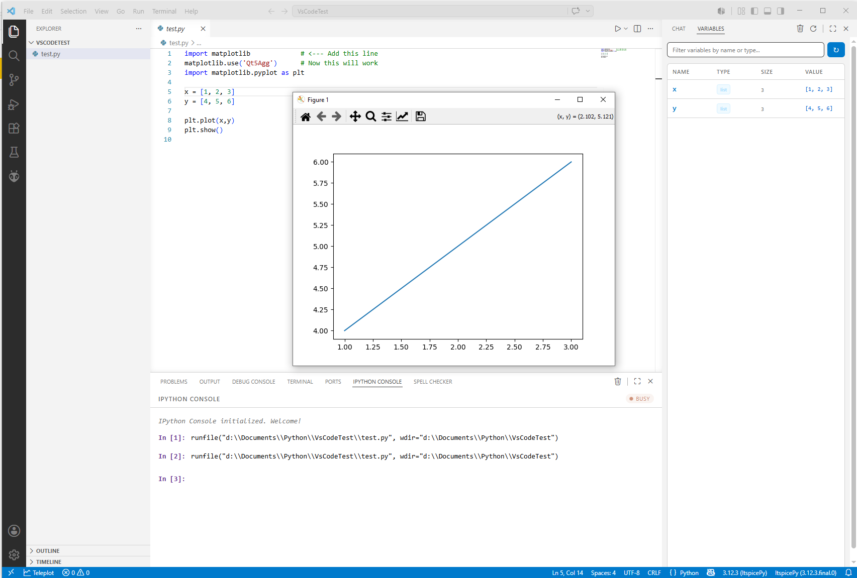
Configuring Visual Studio Code to look like Spyder
In this short post, I will go over the steps I use to make Visual Studio Code (VSCode) act a little more like Spyder. Overall, Spyder is a great IDE for developing Python code. It is basically the MATLAB of the Python world. However, I find that its code suggestions, linting, and other features (like AI 🤮) are lacking. I also find myself using VSCode for other programming tasks, and it is just nice to have one IDE for everything. As a result, I spent some time exploring how to make it act and look a little more like Spyder.
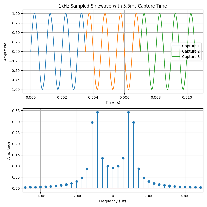
FFT with Python
In this post, I’ll walk through the basics of creating and plotting a discrete-time signal, then show how to analyze it in the frequency domain using the Fast Fourier Transform (FFT). Understanding how a signal behaves in both the time and frequency domains is a key skill in digital signal processing, and the FFT is one of the most powerful tools for doing that.
We’ll start by building a simple signal in Python, visualize it, and then compute its frequency spectrum. From there, we’ll run into a common and sometimes confusing issue called spectral leakage. It’s an important concept that affects how you interpret frequency-domain plots, especially when working with real-world signals. To address spectral leakage, we’ll introduce windowing, a technique that tapers the edges of the signal before performing the FFT. We’ll explore a few popular window types, understand how they work, and see their effects through practical examples.
This post is meant to be hands-on and applied.
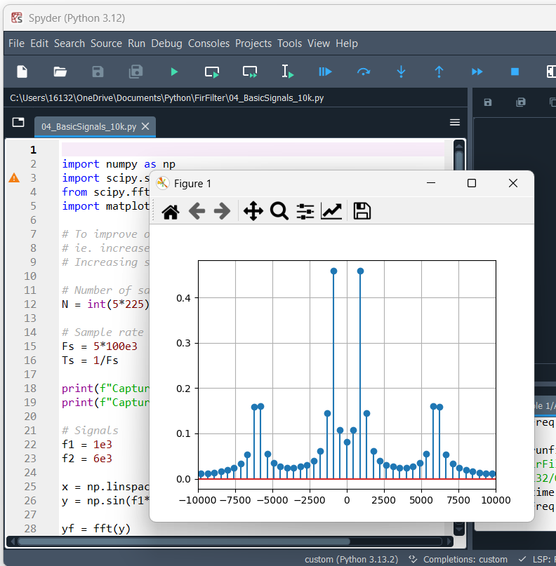
Using Spyder with Python Virtual Environment
In this post, I’ll walk you through how I set up my Spyder IDE to use a Python virtual environment and enable interactive plots with ipympl.
Spyder is a great IDE for scientific and engineering applications in Python - especially if you're coming from a Matlab background. Its interface closely resembles Matlab, making it easier to work with arrays, matrices, and plots compared to something like Visual Studio Code. This is particularly helpful when analyzing data during debugging or after your code runs.