Cooking LTspice with Python

Python logo cooking LTspice in frying pan

Did you know that you can use Python to automate and improve your workflow when simulating circuits in LTspice? It’s surprisingly straightforward, and it opens up a wide range of possibilities. LTspice is a powerful and free SPICE simulator that has been a staple in the electronics world for years, but it hasn’t seen many major updates or modern integrations. That’s where Python comes in.

By combining LTspice with Python, you can script your simulations, sweep parameters, analyze results, and even generate plots automatically. Whether you’re running repetitive simulations, batch processing netlists, or just want to organize your results more effectively, Python can save you time and reduce errors.

In this post, I’ll walk through how to set up a simple Python script that runs an LTspice simulation, extracts data from the raw output files, and displays results in a clean, customizable way. It’s a great way to bring new life to an old but dependable tool, and it can be a game-changer if you’re doing a lot of circuit simulation work.


Before starting I am using Python 3.13 along with the following libraries:

  • Numpy for array handling, math, and plotting

  • Matplotlib for plotting

  • PyLTspice for controlling LTspice and manipulating .net and .raw files

We will also import these libraries to help us manage delays and files

  • Time for delaying the script as we will sometimes need to wait for tasks to complete before executing the next command

  • OS for deleting old generated files

  • Shutil for copying files to different folders

For my IDE, I’m using Spyder, since its layout is very similar to Matlab, which makes it great for this. To see how I setup my workspace see Using Spyder with Python Virtual Environment.

Lets start by importing our required libraries for this tutorial:

import numpy as np
import matplotlib.pyplot as plt
import PyLTSpice

import time
import os
import shutil

Reading RAW Files

We will start with the most basic operation: using Python to read the RAW files generated by an LTspice simulation. These RAW files contain all the node voltages, currents, and time or frequency data produced by the simulation. Note that this data is referred to as traces. For example, the voltage at the output node is represented by the trace V(out).

To begin we will run a transient simulation of the simple RC circuit below.

Simple RC circuit

The LTspice file that contains this circuit is called RC.asc. When we simulate the circuit, LTspice generates several files, including RC.raw, which contains the simulation traces we want to plot.

Image of LTspice related files in a folder with the RAW file highlighted

Next we will use Python to read to contents of RC.raw and plot the V(out) trace vs time. This is done using PyLTSpice’s RawRead class:

ltraw = PyLTSpice.RawRead( RawFileNameLocation )

Where RawFileNameLocation is the location of the raw file that we want to read, and ltraw is the object that holds the traces. In our example we want to read the RC.raw file:

ltraw = PyLTSpice.RawRead("./RC.raw")

From here we now need to extract the desired traces from our ltraw variable using get_trace( ) and get_wave( ):

trace = ltraw.get_trace( dataTraceName ).get_wave( step )

Here, dataTraceName refers to the name of the trace, such as V(out), I(R1), and so on. The step parameter specifies which instance of that trace to retrieve if a step simulation was performed. Since we did not perform a step simulation, we set step = 0. In our example we want to extract the trace data for time and V(out):

xTime = ltraw.get_trace("time").get_wave(0)
yVolt = ltraw.get_trace("V(out)").get_wave(0)

Putting all of this code together, we can plot the V(out) trace as shown below.

# Read the .raw file
ltraw = PyLTSpice.RawRead("./RC.raw")

# Get the x and y data from the raw file
xTime = ltraw.get_trace("time").get_wave(0)
yVolt = ltraw.get_trace("V(out)").get_wave(0)

# Plot the data
plt.figure()
plt.plot(xTime, yVolt, label="C1 = 10nF")
plt.xlabel("Time (s)")
plt.ylabel("Voltage (V)")
plt.title("LTspice Simulation: V(out)")
plt.legend()
plt.grid()
plt.show()
Plotting the trace data from the LTspice RAW file of a RC circuit

Comparing Different Simulations

In the first section, all we did was read a RAW file and plot the results. You might be thinking, "So what?" Well, one limitation of LTspice is that it doesn’t provide a built-in way to store and overlay old simulation results with new ones for direct comparison.

Suppose we take the simple RC circuit from the previous section and add a 10 kΩ load resistor to it. As expected, this load will affect the behavior of the circuit. To address this, we might buffer the RC output using an op-amp. Naturally, we’d want to compare the circuit’s performance with and without the buffer, both in transient and AC analysis.

LTspice does offer some workarounds for these kinds of comparisons. The most common method is to place both circuit versions on the same schematic and simulate them together. This is manageable for small circuits, like the one in this example. However, for larger designs, it becomes tedious and error-prone. For instance, you need to carefully rename all net labels to avoid accidentally connecting the two circuits at shared nodes. This approach also doesn't work well for certain simulation types, such as noise analysis.

Showing how you would have to compare two different circuits in LTspice

Alternatively we can keep these two circuits as separate schematics, simulate them with LTspice and then with Python merge the traces in their respective RAW files together onto a single plot.

So in this example I have two schematics called ResistorDivide.asc and ResistorDivide_Buff.asc which have been simulated in LTspice which generated their respective RAW files. Using the code below, we can plot both V(out) traces to compare the two.

# Read the .raw file
ltraw = PyLTSpice.RawRead("./ResistorDivide.raw")

# Get the x and y data from raw file
xTime = ltraw.get_trace("time").get_wave(0)
yVolt = ltraw.get_trace("V(out)").get_wave(0)

# Plot data
plt.figure()
plt.plot(xTime, yVolt, label="RC")
plt.show()

# Read the .raw file
ltraw = PyLTSpice.RawRead("./ResistorDivide_Buff.raw")

# Get the x and y data from raw file
xTime = ltraw.get_trace("time").get_wave(0)
yVolt = ltraw.get_trace("V(out)").get_wave(0)

# Plot data
plt.plot(xTime, yVolt, label="Buffered")
plt.xlabel('Time (s)')
plt.ylabel('Voltage (V)')
plt.title('LTspice Simulation: V(out)')
plt.legend()
plt.grid()
plt.show()
Plot in Python comparing the two different LTspice schematics after reading their individual RAW files for comparison

Running Simulations

It can be a bit tedious to open each schematic in LTspice, run the simulations manually, and then use Python to plot the results. Fortunately, the PyLTSpice library also allows us to automate simulation using the SimRunner( ) and SpiceEditor( ) classes.

Before diving into the code, I want to point out a small but important detail. There is a brief delay between the time LTspice finishes the simulation and when the RAW file becomes available for Python to read. This introduces two potential issues:

  1. The RAW file may not exist yet or not finished being written when Python tries to access it.

  2. The RAW file is there but it was from the previous simulation.

We’ll need to account for this to avoid reading the wrong file or encountering an error. To keep things straightforward, I’ll first walk you through the basic setup for running a simulation using PyLTSpice. After that, we’ll look at how to handle this timing issue reliably.

There are four steps that are needed to perform the simulation:

  1. Create a handler for LTspice operations (SimRunner)

  2. Create a netlist from your .asc LTspice schematic

  3. Create a handler for this new netlist (SpiceEditor)

  4. Run the LTspice simulation

1. We will start by defining the location of the LTspice executable on your PC:

simulatorLocation = r"D:\Programs\LTspice\LTspice.exe"

This is the location of LTspice.exe on my PC.

Next we will create a SimRunner object called ltsim to handle the LTspice specific operations:

ltsim = PyLTSpice.SimRunner(output_folder= outFolderLocation, simulator= simulatorLocation )

Where outFolderLocation is the folder that you want the generated RAW and .net files that are generated by SimRunner to be saved in. The simulatorLocation is the location of the LTspice.exe executable on your PC. In this example, we will have the generated outputs saved in a temporary folder called temp and the simulator location has already been defined in the simulatorLocation variable.

ltsim = PyLTSpice.SimRunner(output_folder='./temp', simulator=simulatorLocation )

2. Next we will use ltsim to create a netlist used for the actual LTspice simulation:

ltsim.create_netlist( schematicASC )

Where schematicASC is the name of your LTspice .asc schematic file. For example:

ltsim.create_netlist(r'./ResistorDivide.asc')

3. Now we will use the SpiceEditor class to create a handler for the newly created netlist called netlist:

netlist = PyLTSpice.SpiceEditor( schematicNET )

Where schematicNET is the name of your newly created netlist. This should have the same name as your schematicASC but with the .net extension. In our example this looks like:

netlist = PyLTSpice.SpiceEditor(r'./ResistorDivide.net')

4. Finally we call the run( ) function to run the simulation:

ltsim.run(netlist)

We can then use the RawRead( ) function to read the RAW file and plot the traces like we did above.

NOTE: the generated RAW files will have a suffix of “_1” . If you were running multiple simulations this suffix will increment.

Putting this all together and our code looks like the following:

# Location of the LTspice application
simulatorLocation  = r"D:\Programs\LTspice\LTspice.exe"

# Create a handler to perform LTspice specific operations
# Set the location of outputted files into a temp folder
ltsim = PyLTSpice.SimRunner(output_folder='./temp', simulator=simulatorLocation)

# Create a netlist from the LTspice schematic
ltsim.create_netlist(r'./ResistorDivide.asc')

# Create a handler for the newly created netlist
netlist = PyLTSpice.SpiceEditor(r'./ResistorDivide.net')

# Run LTspice simulation of netlist
ltsim.run(netlist)

# Read RAW file for trace data
ltraw = PyLTSpice.RawRead("./temp/ResistorDivide_1.raw")

# Get the x and y data from raw file
xTime = ltraw.get_trace("time").get_wave(0)
yVolt = ltraw.get_trace("V(out)").get_wave(0)

# Plot data
plt.figure()
plt.plot(xTime, yVolt, label="RC")
plt.xlabel('Time (s)')
plt.ylabel('Voltage (V)')
plt.title('LTspice Simulation: V(out)')
plt.legend()
plt.grid()
plt.show()

As I mentioned above there is a bit of a delay between ltsim.run( ) completing and when the RAW file actually is finished being created. To prevent file not found errors, we will wrap the RawRead in a while loop + try statement. If the file is not avaliable yet, we will wait 0.1s and then try again. If this fails more than 10 time, we give up and let Python error out. For longer simulations you may choose to increase the number of attempts or sleep time.

# There seems to be a delay between the ltsim.run() function completing
# and when the new RAW file of the simulation is created. As a result, 
# we will try and read the generated RAW file but if it is not avaliable
# we shall wait until it is there or when we exceed the number of tries.
timeoutTry = 0
while timeoutTry < 10:
    try:
        # Read RAW file
        ltraw = PyLTSpice.RawRead("./temp/ResistorDivide_1.raw")
        break
    
    # RAW file not avaliable
    except:
        timeoutTry += 1
        # Wait
        time.sleep(0.1)

The last concern with this delay after the ltsim.run( ) is that we could accedentally read in an old RAW file with the same name. Since we are putting all the generated files in a temporary folder called temp, I am going to delete all of these files before running any of this code.

# Remove all files from temp folder
def clearTempFiles():
    folder = './temp'

    for filename in os.listdir(folder):
        filepath = os.path.join(folder, filename)
        if os.path.isfile(filepath):
            os.remove(filepath)
            
# Remove old temporary files to prevent Python reading old RAW files
# with the same name as the new ones. There is a delay between running
# the LTspice simulation and the new RAW file being generated
clearTempFiles()

Now putting everything together we get the following script:

# Remove old temporary files to prevent Python reading old RAW files
# with the same name as the new ones. There is a delay between running
# the LTspice simulation and the new RAW file being generated
clearTempFiles()

# Location of the LTspice application
simulatorLocation  = r"D:\Programs\LTspice\LTspice.exe"

# Create a handler to perform LTspice specific operations
# Set the location of outputted files into a temp folder
ltsim = PyLTSpice.SimRunner(output_folder='./temp', simulator=simulatorLocation)

# Create a netlist from the LTspice schematic
ltsim.create_netlist(r'./ResistorDivide.asc')

# Create a handler for the newly created netlist
netlist = PyLTSpice.SpiceEditor(r'./ResistorDivide.net')

# Run LTspice simulation of netlist
ltsim.run(netlist)

# There seems to be a delay between the ltsim.run() function completing
# and when the new RAW file of the simulation is created. As a result, 
# we will try and read the generated RAW file but if it is not avaliable
# we shall wait until it is there or when we exceed the number of tries.
timeoutTry = 0
while timeoutTry < 10:
    try:
        # Read RAW file
        ltraw = PyLTSpice.RawRead("./temp/ResistorDivide_1.raw")
        break
    # RAW file not avaliable
    except:
        timeoutTry += 1
        # Wait
        time.sleep(0.1)

# Get the x and y data from raw file
xTime = ltraw.get_trace("time").get_wave(0)
yVolt = ltraw.get_trace("V(out)").get_wave(0)

# Plot data
plt.figure()
plt.plot(xTime, yVolt, label="RC")
plt.xlabel('Time (s)')
plt.ylabel('Voltage (V)')
plt.title('LTspice Simulation: V(out)')
plt.legend()
plt.grid()
plt.show()
Plot of RC circuit output after Python performed LTspice simulation

Running Multiple Simulations to Compare Results

Basically we are going to repeat Application 1 but instead of us manually simulating from LTspice and then using Python to read traces out of the RAW files, we will do everything automatically from within Python.

To do this we will basically duplicate the above code from the Running Simulations section but

  • ltsim.create_netlist( ) generates a .net file using the .asc file of the new schematic

  • netlist = PyLTSpice.SpiceEditor( ) configures to use the newly generated .net file

  • ltraw = PyLTSpice.RawRead( ) reads the newly simulated .net file with the suffix “_2” because it is the second time we have run an LTspice simulation

Putting this all together gives the following code:

# Remove all files from temp folder
def clearTempFiles():
    folder = './temp'

    for filename in os.listdir(folder):
        filepath = os.path.join(folder, filename)
        if os.path.isfile(filepath):
            os.remove(filepath)

# Remove old temporary files to prevent Python reading old RAW files
# with the same name as the new ones. There is a delay between running
# the LTspice simulation and the new RAW file being generated
clearTempFiles()

# Location of the LTspice application
simulatorLocation  = r"D:\Programs\LTspice\LTspice.exe"

# Create a handler to perform LTspice specific operations
# Set the location of outputted files into a temp folder
ltsim = PyLTSpice.SimRunner(output_folder='./temp', simulator=simulatorLocation)

#### Simulate RC circuit ####

# Create a netlist from the LTspice schematic
ltsim.create_netlist(r'./ResistorDivide.asc')

# Create a handler for the newly created netlist
netlist = PyLTSpice.SpiceEditor(r'./ResistorDivide.net')

# Run LTspice simulation of netlist
ltsim.run(netlist)

# Wait for the RAW file to appear
timeoutTry = 0
while timeoutTry < 10:
    try:
        # Read RAW file
        ltraw = PyLTSpice.RawRead("./temp/ResistorDivide_1.raw")
        break
    except:
        timeoutTry += 1
        # Wait
        time.sleep(0.1)

# Get the x and y data from raw file
xTime = ltraw.get_trace("time").get_wave(0)
yVolt = ltraw.get_trace("V(out)").get_wave(0)

# Plot data
plt.figure()
plt.plot(xTime, yVolt, label="RC")
plt.show()

#### Simulate Buffered RC circuit ####

ltsim.create_netlist(r'./ResistorDivide_Buff.asc')
netlist = PyLTSpice.SpiceEditor(r'./ResistorDivide_Buff.net')
ltsim.run(netlist)

timeoutTry = 0
while timeoutTry < 10:
    try:
        ltraw = PyLTSpice.RawRead("./temp/ResistorDivide_Buff_2.raw")
        break
    except:
        timeoutTry += 1
        # Wait
        time.sleep(0.1)

xTime_buf = ltraw.get_trace("time").get_wave(0)
yVolt_buf = ltraw.get_trace("V(out)").get_wave(0)

# Plot data
plt.plot(xTime_buf, yVolt_buf, label="RC Buffered")
plt.xlabel('Time (s)')
plt.ylabel('Voltage (V)')
plt.title('LTspice Simulation: V(out)')
plt.legend()
plt.grid()
plt.tight_layout()
plt.show()
Plot of trace data of two different circuits to compare results. Python had been used to run simulations.

You will notice that we could be a lot more efficient with our code if we

  • Create a list of schematics that we want to simulate and add a for loop to simulate them all

  • Have a variable to keep track of the simulation number for the RAW file suffix number

So with this simple change, we can run multiple simulations at the same time by simply adding the schematic name to the list of schematics (called schematicName in script below).

# Remove all files from temp folder
def clearTempFiles():
    folder = './temp'

    for filename in os.listdir(folder):
        filepath = os.path.join(folder, filename)
        if os.path.isfile(filepath):
            os.remove(filepath)

# Remove old temporary files to prevent Python reading old RAW files
# with the same name as the new ones. There is a delay between running
# the LTspice simulation and the new RAW file being generated
clearTempFiles()

# Location of the LTspice application
simulatorLocation  = r"D:\Programs\LTspice\LTspice.exe"

# Create a handler to perform LTspice specific operations
# Set the location of outputted files into a temp folder
ltsim = PyLTSpice.SimRunner(output_folder='./temp', simulator=simulatorLocation)

# List of schematic names to be simulated
schematicName = ["ResistorDivide", 
                 "ResistorDivide_Buff", 
                 "ResistorDivide_Large-RL", 
                 "ResistorDivide_Small-R1"]

# Variable to keep track of the RAW file suffix number
simNumber = 0

# Create empty plot
plt.figure()

# For each schematic that we want to simulate
for schematic in schematicName:
    
    # Increment the simulation number for the RAW file suffix
    simNumber += 1
    
    # Create a netlist from the LTspice schematic
    ltsim.create_netlist('.\\' + schematic + '.asc')
    
    # Create a handler for the newly created netlist
    netlist = PyLTSpice.SpiceEditor('.\\' + schematic + '.net')
    
    # Run LTspice simulation of netlist
    ltsim.run(netlist)
    
    # Wait for the RAW file to appear
    timeoutTry = 0
    while timeoutTry < 10:
        try:
            # Read RAW file
            ltraw = PyLTSpice.RawRead('.\\temp\\' + schematic + '_' + str(simNumber) +  '.raw')
            break
        except:
            timeoutTry += 1
            # Wait
            time.sleep(0.1)

    # Get the x and y data from raw file
    xTime = ltraw.get_trace("time").get_wave(0)
    yVolt = ltraw.get_trace("V(out)").get_wave(0)
    
    # Plot data
    plt.plot(xTime, yVolt, label=schematic)
    plt.show()

# Plot data
plt.xlabel('Time (s)')
plt.ylabel('Voltage (V)')
plt.title('LTspice Simulation: V(out)')
plt.legend()
plt.grid()
plt.tight_layout()
plt.show()
Plot showing the output traces of many different LTspice schematics to compare results

I should note that this is different than running a step simulation because we could be simulating vastly different schematics at the same time (as opposed to just changing one or two parameters in the same schematic).

Step Simulations

Simple step simulations where we step through a single parameter are pretty trivial in LTspice. Unfortunately, at this time of writing, I would say that the PyLTspice library does a poor job at handling step simulations. However I will still show you the process of setting up a step simulation in Python as it shows some new powerful functions that we will use extensively going forward.

For this demo, we will use the following schematic of a multiple feedback second-order filter:

Schematic of a multiple feedback second-order filter used for simulation example

To perform the step simulation we will need to perform the following steps:

  1. Adjust the netlist so that R3’s value to be the variable/parameter called Res3

  2. Define the parameter Res3 in the netlist

  3. Add the .step instruction to the netlist in order to perform a step simulation

  4. Manually calculate Res3’s step values for plotting

  5. Plotting the step simulation

1. For the step simulation we are going to change the value of the R3 resistor to a variable/parameter called Res3. We can do this by changing the component value in the netlist:

netlist.set_component_value( componentName , value )

Where componentName is the name or reference designator of the component, and the value is the value parameter of the component that we are changing to. In our example it looks like:

netlist.set_component_value('R3', '{Res3}')

and {Res3} is the variable/parameter that we will change in the step simulation.

2. We still need to define the parameter {Res3} and we can do that using:

netlist.set_parameter( parameterName , value)

Where parameterName is the name of our parameter and value is the value of the parameter. In our example this looks like:

netlist.set_parameter('Res3',1.4e3)

3. Now we will add the instruction for the step simulation, changing the value of R3 from 1.4k ohm to 14k ohm with increments of 1k ohm:

netlist.add_instruction('.step param Res3 1.4k 14k 1k')

4. This is the annoying part / error prone. We need to manually calculate the value of R3 for each of the steps. For whatever reason the PyLTspice library does not have a function that gives us the value of R3 for each step simulation. As a result, we will use python to calculate this using numpy’s arange function and then we have to add the last point in our step function to this array because LTspice will always simulate the stop value in the step simulation:

res3_values = np.arange(1.4e3,14e3,1e3)
res3_values = np.append(res3_values, 14e3)

I stress that this is an issue with the PyLTspice library because it can be error prone. Also we could configure the step simulation to use logarithmic steps instead of linear, further increasing the likelihood of error.

5. To plot the traces from the step simulation we will create a for loop that cycles through each step. We will use the step number to select the correct step trace using the .get_wave( ) function. Since this is an AC simulation we will be using the frequency trace for the x-axis and we will convert V(out) to dB:

# For each step in the simulation, plot the corresponding trace
for step in simSteps:
    
    # Get the x and y data from raw file
    xFreq = ltraw.get_trace("frequency").get_wave(step)
    yVolt = ltraw.get_trace("V(out)").get_wave(step)
    
    # Plot trace. Note we are converting data into dB
    plt.plot(xFreq, 20*np.log10(np.abs(yVolt)), label=res3_values[step])
    plt.show()

Putting all of the code together we get the following:

# Remove all files from temp folder
def clearTempFiles():
    folder = './temp'

    for filename in os.listdir(folder):
        filepath = os.path.join(folder, filename)
        if os.path.isfile(filepath):
            os.remove(filepath)

# Remove old temporary files to prevent Python reading old RAW files
# with the same name as the new ones. There is a delay between running
# the LTspice simulation and the new RAW file being generated
clearTempFiles()

# Location of the LTspice application
simulatorLocation  = r"D:\Programs\LTspice\LTspice.exe"
# Name of the schematic
schematic = 'MFB'

# Create a handler to perform LTspice specific operations
# Set the location of outputted files into a temp folder
ltsim = PyLTSpice.SimRunner(output_folder='./temp', simulator=simulatorLocation)

# Create a netlist from the LTspice schematic
ltsim.create_netlist('.\\' + schematic + '.asc')

# Create a handler for the newly created netlist
netlist = PyLTSpice.SpiceEditor('.\\' + schematic + '.net')

# Adjust netlist components, parameters, and instructions to perform step simulation

# Change resistor R3 to be a parameter
netlist.set_component_value('R3', '{Res3}')
# Define the initial value of this parameter
netlist.set_parameter('Res3',1.4e3)
# Add instruction to do a step simulation based on this parameter
netlist.add_instruction('.step param Res3 1.4k 14k 1k')

# Manually calculate the step values for our plot legend 
# pyLTspice seems to not be able to exctract the values of the parameter
# from the raw file trace data
res3_values = np.arange(1.4e3,14e3,1e3)
res3_values = np.append(res3_values, 14e3) # Add final step value to array

# Run LTspice simulation of netlist
ltsim.run(netlist)

# There seems to be a delay between the ltsim.run() function completing
# and when the new RAW file of the simulation is created. As a result, 
# we will try and read the generated RAW file but if it is not avaliable
# we shall wait until it is there or when we exceed the number of tries.
timeoutTry = 0
while timeoutTry < 10:
    try:
        # Read RAW file
        ltraw = PyLTSpice.RawRead('.\\temp\\' + schematic + '_1.raw')
        break
    # RAW file not avaliable
    except:
        timeoutTry += 1
        # Wait
        time.sleep(0.1)

# Empty plot
plt.figure()

# Get the number of steps from LTspice simulation
simSteps = ltraw.get_steps()

# For each step in the simulation, plot the corresponding trace
for step in simSteps:
    
    # Get the x and y data from raw file
    xFreq = ltraw.get_trace("frequency").get_wave(step)
    yVolt = ltraw.get_trace("V(out)").get_wave(step)
    
    # Plot trace. Note we are converting data into dB
    plt.plot(xFreq, 20*np.log10(np.abs(yVolt)), label=res3_values[step])
    plt.show()

plt.xscale("log")
plt.xlabel('Frequency (Hz)')
plt.ylabel('Gain (dB)')
plt.title('LTspice Simulation: V(out)')
plt.legend()
plt.grid()
plt.tight_layout()
plt.show()
Plot of step simulation where we varry a resistor size

I hope I have highlighted that using the build-in step simulation function of PyLTspice is a bit broken.

Fortunately there is just a better way to do these step simulations by simply using the set_component_value ( ) function to set the value of the component, run the simulation, plot, change the value of the component, and repeat.

So in our example we will remove:

netlist.set_parameter('Res3',1.4e3)
netlist.add_instruction('.step param Res3 1.4k 14k 1k')

We will create an array with the values of R3 using:

res3_values = np.arange(1.4e3,14e3,1e3)

Then we use a for loop to simulate through each of the different R3 values. The loop will consist of the following operations:

  1. Increment the simNumber to keep track of the RAW file’s “_1” suffix

  2. Set the R3 component value

  3. Run the simulation

  4. Read the RAW file

  5. Plot the trace

Putting all of this together and our code looks like:

# Remove all files from temp folder
def clearTempFiles():
    folder = './temp'

    for filename in os.listdir(folder):
        filepath = os.path.join(folder, filename)
        if os.path.isfile(filepath):
            os.remove(filepath)

# Remove old temporary files to prevent Python reading old RAW files
# with the same name as the new ones. There is a delay between running
# the LTspice simulation and the new RAW file being generated
clearTempFiles()

# Location of the LTspice application
simulatorLocation  = r"D:\Programs\LTspice\LTspice.exe"
# Name of the schematic
schematic = 'MFB'

# Create a handler to perform LTspice specific operations
# Set the location of outputted files into a temp folder
ltsim = PyLTSpice.SimRunner(output_folder='./temp', simulator=simulatorLocation)

# Create a netlist from the LTspice schematic
ltsim.create_netlist('.\\' + schematic + '.asc')

# Create a handler for the newly created netlist
netlist = PyLTSpice.SpiceEditor('.\\' + schematic + '.net')

# Array of R3 values
res3_values = np.arange(1.4e3,14e3,1e3)

# Empty plot
plt.figure()

# Variable to keep track of the RAW file suffix number
simNumber = 0

# For each step in the simulation, plot the corresponding trace
for res3 in res3_values:

    # Increment the simulation number for the RAW file suffix
    simNumber += 1

    # Change resistor R3 to be a parameter
    netlist.set_component_value('R3', str(res3))

    # Run LTspice simulation of netlist
    ltsim.run(netlist)

    # There seems to be a delay between the ltsim.run() function completing
    # and when the new RAW file of the simulation is created. As a result, 
    # we will try and read the generated RAW file but if it is not available
    # we shall wait until it is there or when we exceed the number of tries.
    timeoutTry = 0
    while timeoutTry < 10:
        try:
            # Read RAW file
            ltraw = PyLTSpice.RawRead('.\\temp\\' + schematic + '_' + str(simNumber) +  '.raw')
            break

        except: # RAW file not available
            timeoutTry += 1
            # Wait
            time.sleep(0.1)

    # Get the x and y data from raw file
    xFreq = ltraw.get_trace("frequency").get_wave(0)
    yVolt = ltraw.get_trace("V(out)").get_wave(0)

    # Plot trace. Note we are converting data into dB
    plt.plot(xFreq, 20*np.log10(np.abs(yVolt)), label=str(res3))
    plt.show()

plt.xscale("log")
plt.xlabel('Frequency (Hz)')
plt.ylabel('Gain (dB)')
plt.title('LTspice Simulation: V(out)')
plt.legend()
plt.grid()
plt.tight_layout()
plt.show()

And it produces more or less the same step plot as shown above.

Step Symbol Models

Like we stepped through resistor values, we can also step through symbol models which is something you cannot do with LTspice (as far as I know).

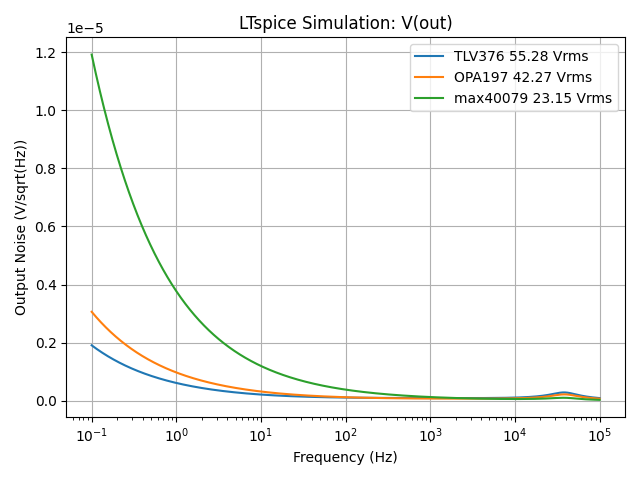
In this example we will take multiple feedback second-order filter from the last section and simulate the output noise of the circuit with TLV376, OPA197, and MAX40079 opamps.

Schematic of a multiple feedback second-order filter used for simulation example

We will start by making a list with the file names of our opamp models:

opampModels = ['TLV376.cir', 'OPA197.cir', 'max40079.lib']

Then we will use the set_element_model( ) to change the model of the opamp:

netlist.set_element_model( symbolName , model )

Where symbolName is the name/reference designator of the symbol and model is the name of the model you want to use. For example:

netlist.set_element_model('XU1', opampModels[:-4])

With XU1 being the name of the opamp (note that on the LTspice schematic it will just be called U1, but in the netlist there is a prefix X added to the name) and opampModels is our list of opamp models. Note that our opampModels list include the extension for the model but we will remove this extension using [:-4] to only leave us with the text name of the opamp model.

This is almost everything that you need to do, however since we are saving all of our generated netlists and RAW files inside a folder called temp when we define ltsim

ltsim = PyLTSpice.SimRunner(output_folder='./temp', simulator=simulatorLocation)

We need to also put these models inside the temp folder. This is accomplished using the shutil library to copy these models into the temp folder:

shutil.copy( source , destination )

Where source is the file we want to copy and destination is where we want to copy the file to. In our case:

shutil.copy('.\\' + opamp, '.\\temp\\' + opamp)


For fun we will also calculate the total RMS output noise from the simulation data (as uVrms):

rmsNoise_uV = np.sqrt(np.trapezoid(yVolt**2, xFreq)) * 10**6

And plot this information in the plot ledgend:

plt.plot(xFreq, yVolt, label=opamp[:-4] + ' '+ f"{rmsNoise_uV:.2f}" + ' Vrms')


Putting all of this code together and we get:

# Remove all files from temp folder
def clearTempFiles():
    folder = './temp'

    for filename in os.listdir(folder):
        filepath = os.path.join(folder, filename)
        if os.path.isfile(filepath):
            os.remove(filepath)

# Remove old temporary files to prevent Python reading old RAW files
# with the same name as the new ones. There is a delay between running
# the LTspice simulation and the new RAW file being generated
clearTempFiles()

# Location of the LTspice application
simulatorLocation  = r"D:\Programs\LTspice\LTspice.exe"
# Name of the schematic
schematic = 'MFB_OpampTest'

# Create a handler to perform LTspice specific operations
# Set the location of outputted files into a temp folder
ltsim = PyLTSpice.SimRunner(output_folder='./temp', simulator=simulatorLocation)

# Create a netlist from the LTspice schematic
ltsim.create_netlist('.\\' + schematic + '.asc')

# Create a handler for the newly created netlist
netlist = PyLTSpice.SpiceEditor('.\\' + schematic + '.net')

# Array of opamps
opampModels = ['TLV376.cir', 'OPA197.cir', 'max40079.lib']

# Empty plot
plt.figure()

# Variable to keep track of the RAW file suffix number
simNumber = 0

# For each step in the simulation, plot the corresponding trace
for opamp in opampModels:

    # Increment the simulation number fo the RAW file suffix
    simNumber += 1

    # Change resistor R3 to be a parameter
    netlist.set_element_model('XU1', opamp[:-4])
    netlist.add_instruction('.lib ' + opamp)

    # Since the LTspice simulation will occur in the temp folder
    # We need to put the opamp model there as well
    # We are copying the model from out "main" folder to the temp folder
    shutil.copy('.\\' + opamp, '.\\temp\\' + opamp)

    # Run LTspice simulation of netlist
    ltsim.run(netlist)

    # There seems to be a delay between the ltsim.run() function completing
    # and when the new RAW file of the simulation is created. As a result,
    # we will try and read the generated RAW file but if it is not avaliable
    # we shall wait until it is there or when we exceed the number of tries.
    timeoutTry = 0
    while timeoutTry < 10:
        try:
            # Read RAW file
            ltraw = PyLTSpice.RawRead('.\\temp\\' + schematic + '_' + str(simNumber) +  '.raw')
            break

        except: # RAW file not avaliable
            timeoutTry += 1
            # Wait
            time.sleep(0.1)

    # Get the x and y data from raw file
    xFreq = ltraw.get_trace("frequency").get_wave(0)
    yVolt = ltraw.get_trace("V(onoise)").get_wave(0)

    # Calculate total RMS noise in uV
    rmsNoise_uV = np.sqrt(np.trapezoid(yVolt**2, xFreq)) * 10**6

    # Plot trace.
    plt.plot(xFreq, yVolt, label=opamp[:-4] + ' '+ f"{rmsNoise_uV:.2f}"  + ' Vrms')
    plt.show()

plt.xscale("log")
plt.xlabel('Frequency (Hz)')
plt.ylabel('Output Noise (V/sqrt(Hz))')
plt.title('LTspice Simulation: V(out)')
plt.legend()
plt.grid()
plt.tight_layout()
plt.show()
A plot of a "Step" simulation where we are stepping through different opamp models

Custom Input Signals

Another nice feature with using Python and LTspice together is that we can easily create custom signals in python and then feed them into LTspice. This is accomplished by:

  1. Creating the custom signal in Python

  2. Saving the custom signal as a PWL file (has extension .txt still)

  3. Changing the "model” of our voltage source to a PWL file that is then linked to our newly created PWL file with custom signal

For this example, lets take our multiple feedback second-order filter

Schematic of a multiple feedback second-order filter used for simulation example

We are going to first convert the simulation type from AC to transient using the add_instruction( ) function that we have used before:

netlist.add_instruction('.tran 5m')

Next we are going to create the x and y data for our custom signal:

xTime = np.linspace(0, 5e-3,1000)

yVolt = 0.5*np.sin(2*np.pi*xTime*1e3) + 0.5*np.sin(2*np.pi*xTime*4e3)

Now we will use the following function to take this x and y data and save it as a PWL file

# Create a PWL file with x,y data
def save_pwl_file(x, y, filename):
    with open(filename, 'w') as f:
        for t, v in zip(x, y):
            f.write(f"{t:.9g}\t{v:.9g}\n")

Which we call to create our PWL text file called pwl_data.txt

save_pwl_file(xTime, yVolt, "pwl_data.txt")

We will also plot this custom input signal on a plot to compare to.

Like we had to do in the Step Symbol Models section, we also need to copy the PWL file to the temp folder with our netlist:

shutil.copy('.\\pwl_data.txt', '.\\temp\\pwl_data.txt')

Putting all of this code together and we get:

# Remove all files from temp folder
def clearTempFiles():
    folder = './temp'

    for filename in os.listdir(folder):
        filepath = os.path.join(folder, filename)
        if os.path.isfile(filepath):
            os.remove(filepath)

# Create a PWL file with x,y data
def save_pwl_file(x, y, filename):
    with open(filename, 'w') as f:
        for t, v in zip(x, y):
            f.write(f"{t:.9g}\t{v:.9g}\n")

# Remove old temporary files to prevent Python reading old RAW files
# with the same name as the new ones. There is a delay between running
# the LTspice simulation and the new RAW file being generated
clearTempFiles()

# Location of the LTspice application
simulatorLocation  = r"D:\Programs\LTspice\LTspice.exe"
# Name of the schematic
schematic = 'MFB'

# Create a handler to perform LTspice specific operations
# Set the location of outputted files into a temp folder
ltsim = PyLTSpice.SimRunner(output_folder='./temp', simulator=simulatorLocation)

# Create a netlist from the LTspice schematic
ltsim.create_netlist('.\\' + schematic + '.asc')

# Create a handler for the newly created netlist
netlist = PyLTSpice.SpiceEditor('.\\' + schematic + '.net')

# Convert our AC simulation to transient
# Note: there is a remove_instruction() but it seems like the add_instruction
# removes the AC simulation directive from the netlist automatically
netlist.add_instruction('.tran 5m')

# Generate custom input signal
xTime = np.linspace(0, 5e-3,1000)
yVolt = 0.5*np.sin(2*np.pi*xTime*1e3) + 0.5*np.sin(2*np.pi*xTime*4e3)

# Plot our custom signal for comparison
plt.figure()
plt.plot(xTime, yVolt, label='Input')
plt.show()

# Save custom input signal as a PWL file
save_pwl_file(xTime, yVolt, "pwl_data.txt")

# Since the LTspice simulation will occur in the temp folder
# We need to put the PWL file there as well
# We are copying the PWL file from our "main" folder to the temp folder
shutil.copy('.\\pwl_data.txt', '.\\temp\\pwl_data.txt')

# Update the input voltage source
netlist.set_element_model('VS', 'PWL file=pwl_data.txt')

# Run LTspice simulation of netlist
ltsim.run(netlist)

# There seems to be a delay between the ltsim.run() function completing
# and when the new RAW file of the simulation is created. As a result,
# we will try and read the generated RAW file but if it is not available
# we shall wait until it is there or when we exceed the number of tries.
timeoutTry = 0
while timeoutTry < 10:
    try:
        # Read RAW file
        ltraw = PyLTSpice.RawRead('.\\temp\\' + schematic + '_1.raw')
        break

    except: # RAW file not available
        timeoutTry += 1
        # Wait
        time.sleep(0.1)

# Get the x and y data from raw file
xTime = ltraw.get_trace("time").get_wave(0)
yVolt = ltraw.get_trace("V(out)").get_wave(0)

# Plot trace
plt.plot(xTime, yVolt, label='Output')
plt.xlabel('Time (s)')
plt.ylabel('Output Voltage (V)')
plt.title('LTspice Simulation: V(out)')
plt.legend()
plt.grid()
plt.tight_layout()
plt.show()
Plot showing the inputted custom signal and the resulting output signal. The custom signal inputted was created in Python and fed into the LTspice simulation

This was a simple example, but theoretically you could also take the simulation output of one LTspice simulation and feed it as an input into another. This could help with convergence issues or allow you to break a large LTspice schematic into smaller parts. Warning: be careful if you do this as you may forget to account for circuit loading effects betweek circuit blocks/schematics.

Writing to RAW Files

We can use PyLTSpice to also write to the RAW files directly. For example, we could create our own custom signal and write it to a RAW file and then view this signal in LTspice. I am not sure how useful it would be.

However, you might want to use Python to step through different symbol models and then be able to use LTspice’s built in tools to compare the plots.

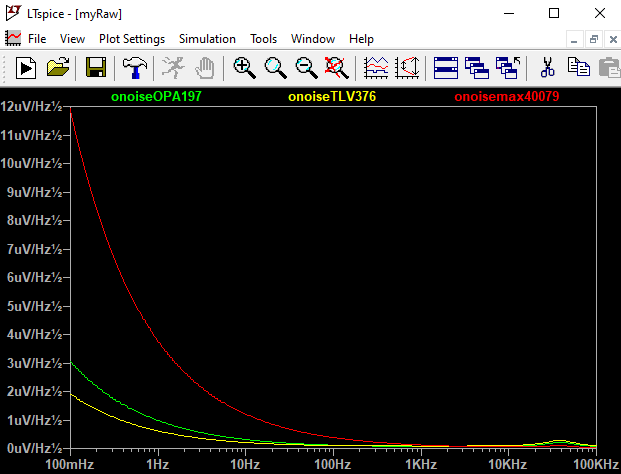
I will admit this is unfortunatly not the easiest thing to do, and I had some problems implementing it. But I will walk you through the multiple feedback second-order filter step simulation with different symbol models that we had performed in the Step Simulation Models section above. The code will almost be exactly the same as before, but we will add additional lines of code to write to the RAW file.

There seems to also be a bit of an order that we need to follow:

  1. Create a handler for the RawWrite class

  2. Define what the simulation type is

  3. Define a plot name (doesn’t seem to always be nessesary but there seems to be a bug in AC analysis where you must call the plot name 'AC Analysis' for it to work)

  4. Write the x axis data first and only once

  5. Write the y data

  6. Save the RAW file

1. Simply create our handler:

ltwrite = PyLTSpice.RawWrite(fastacces=False)

2. Set the simulation type:

ltwrite.simulation_type = type

Where type is the name of the simulation types. For example, we will perform a noise analysis:

ltwrite.simulation_type = 'Noise'

3. We will define a plot name using:

ltwrite.plot_name = plotName

Where plotName is the name of the plot. Note for atleast the AC analysis, there is a specific name in which a plot much be named for its simulation type. For example:

ltwrite.plot_name = 'Noise Spectral Density’

4. Write the x axis by creating a Trace object and then using the add_trace( ) function:

xTrace = PyLTSpice.Trace( traceName , traceData , numerical_type= dataType)
ltwrite.add_trace(xTrace)

Where traceName is the name of the trace (ie. V(out), I(out), time, frequency, etc), traceData is the array which holds our data, and dataType is the type of data (ie. real, double, complex, etc). For our noise simulation example we are going to want to add the frequency trace and its dataType is double:

xTrace = PyLTSpice.Trace('frequency', xFreq, numerical_type='double')
ltwrite.add_trace(xTrace)

5. Identical to what we do with the x axis. In the noise simulation we will use the dataType of real:

yTrace = PyLTSpice.Trace('onoise' + opamp[:-4] , yVolt, numerical_type='real')
ltwrite.add_trace(yTrace)

6. Then to save the RAW file we will use the save( ) function:

ltwrite.save( rawLocation )

Where rawLocation is the location where we want to save the file. For example:

ltwrite.save('.\\temp\\myRaw.RAW')

Putting this all together we get the following code:

# Remove all files from temp folder
def clearTempFiles():
    folder = './temp'

    for filename in os.listdir(folder):
        filepath = os.path.join(folder, filename)
        if os.path.isfile(filepath):
            os.remove(filepath)

# Remove old temporary files to prevent Python reading old RAW files
# with the same name as the new ones. There is a delay between running
# the LTspice simulation and the new RAW file being generated
clearTempFiles()

# Location of the LTspice application
simulatorLocation  = r"D:\Programs\LTspice\LTspice.exe"
# Name of the schematic
schematic = 'MFB_OpampTest'

# Create a handler to perform LTspice specific operations
# Set the location of outputted files into a temp folder
ltsim = PyLTSpice.SimRunner(output_folder='./temp', simulator=simulatorLocation)

# Create a netlist from the LTspice schematic
ltsim.create_netlist('.\\' + schematic + '.asc')

# Create a handler for the newly created netlist
netlist = PyLTSpice.SpiceEditor('.\\' + schematic + '.net')

# Array of opamps
opampModels = ['TLV376.cir', 'OPA197.cir', 'max40079.lib']

# Initialize class to write RAW file
ltwrite = PyLTSpice.RawWrite(fastacces=False)

# Configure the RAW file to be for a Noise simulation
ltwrite.simulation_type = 'Noise'

# Plot name. Important for AC simulation at least.
ltwrite.plot_name = 'Noise Spectral Density’

# Empty plot
plt.figure()

# Variable to keep track of the RAW file suffix number
simNumber = 0

# For each step in the simulation, plot the corresponding trace
for opamp in opampModels:

    # Increment the simulation number for the RAW file suffix
    simNumber += 1

    # Change opamp model in netlist
    netlist.set_element_model('XU1', opamp[:-4])
    netlist.add_instruction('.lib ' + opamp)

    # Copy opamp model to temp folder for LTspice simulation
    shutil.copy('.\\' + opamp, '.\\temp\\' + opamp)

    # Run LTspice simulation of netlist
    ltsim.run(netlist)

    # Wait for RAW file to become available
    timeoutTry = 0
    while timeoutTry < 10:
        try:
            # Read RAW file
            ltraw = PyLTSpice.RawRead('.\\temp\\' + schematic + '_' + str(simNumber) +  '.raw')
            break
        except:
            timeoutTry += 1
            time.sleep(0.1)

    # Get the x and y data from raw file
    xFreq = ltraw.get_trace("frequency").get_wave(0)
    yVolt = ltraw.get_trace("V(onoise)").get_wave(0)

    # Plot trace
    plt.plot(xFreq, yVolt, label=opamp[:-4])
    plt.show()

    # Write trace data to RAW file
    if simNumber == 1:
        xTrace = PyLTSpice.Trace('frequency', xFreq, numerical_type='double')
        ltwrite.add_trace(xTrace)

    yTrace = PyLTSpice.Trace('onoise' + opamp[:-4], yVolt, numerical_type='real')
    ltwrite.add_trace(yTrace)

# Save traces to RAW file
ltwrite.save('.\\temp\\myRaw.RAW')

# Format plot
plt.xscale("log")
plt.xlabel('Frequency (Hz)')
plt.ylabel('Output Noise (V/sqrt(Hz))')
plt.title('LTspice Simulation: V(out)')
plt.legend()
plt.grid()
plt.tight_layout()
plt.show()
Merged multiple traces into a RAW file that could be read and plotted by LTspice's trace viewer

So I will note that figuring which plot name and numerical types to use for each simulation types is difficult to determine. I have used chatGPT to create a table for this purpose. I have tested a few of the simulation types but not all of them.

Simulation Type (simulation_type) Suggested plot_name X-axis Trace (numerical_type) Y-axis Trace (numerical_type)
'Tran'Transient Analysis'double' (e.g., time)'real'
'AC'AC Analysis'complex' (frequency)'complex'
'Noise'Noise Spectral Density'double' (frequency)'real'
'DCTransfer'DC Transfer Curve'double''real'
'DCop' or 'OperatingPoint'DC Operating Point(none or 'double')'real'
'TF'Transfer Function'double''real'
'Sens'Sensitivity Analysis'double''real'
'Distortion'Harmonic Distortion'double' or 'frequency''complex'
'FFT'FFT Analysis'double' (usually time or freq)'complex' or 'real'

Simulation Suite

Probably the most practical use of combinding Python and LTspice together is being able to run multiple types of simulations with one click of the button and having them all plotted side-by-side. In the above sections we have covered everything we need to acomplish this task.

My circuit is yet again the multiple feedback second-order filter circuit and I am going to create a couple lists to keep track of simulation options:

  • simType is a list of simulations that get performed

  • simSpice is the corresponding simulation instructions

  • vsModel is the corresponding settings that the input voltage source (VS) needs to be set to for the simulation

  • xDataName, yDataName are the trace names of the simulation data that I want to plot

I will then create a for loop to cycle through each simulation and plot data in a subplot plot.

Putting this all together we get the following code:

# Remove all files from temp folder
def clearTempFiles():
    folder = './temp'

    for filename in os.listdir(folder):
        filepath = os.path.join(folder, filename)
        if os.path.isfile(filepath):
            os.remove(filepath)

# Remove old temporary files to prevent Python reading old RAW files
# with the same name as the new ones. There is a delay between running
# the LTspice simulation and the new RAW file being generated
clearTempFiles()

# Location of the LTspice application
simulatorLocation  = r"D:\Programs\LTspice\LTspice.exe"
# Name of the schematic
schematic = 'MFB'

# Create a handler to perform LTspice specific operations
# Set the location of outputted files into a temp folder
ltsim = PyLTSpice.SimRunner(output_folder='./temp', simulator=simulatorLocation)

# Create a netlist from the LTspice schematic
ltsim.create_netlist('.\\' + schematic + '.asc')

# Create a handler for the newly created netlist
netlist = PyLTSpice.SpiceEditor('.\\' + schematic + '.net')

# Simulations to perform
simType = ['Transient',
           'AC',
           'Noise',
           'DC']

# Spice instructions to perform corresponding simulation
simSpice = ['.tran 5m',
            '.ac dec 1000 1k 100k',
            '.noise V(out) VS dec 1000 0.1 100k',
            '.dc VS 0 5 0.01']

# Input voltage source (VS) settings
vsModel = ['SINE(2.5 10m 1k)',
           'AC 1',
           '2.5',
           '2.5']

# X axis data to plot
xDataName = ['time',
             'frequency',
             'frequency',
             'vs']

# Y axis data to plot
yDataName = ['V(out)',
             'V(out)',
             'V(onoise)',
             'V(out)']

# Empty plot
fig, axs = plt.subplots(2, 2, figsize=(12, 8))
axs = axs.flatten()

# Variable to keep track of the RAW file suffix number
simNumber = 0

for sim in simType:

    # Update the input voltage source
    netlist.set_element_model('VS', vsModel[simNumber].strip())

    # Set our simulation type
    netlist.add_instruction(simSpice[simNumber])

    # Run LTspice simulation of netlist
    ltsim.run(netlist)

    # Wait for RAW file to become available
    timeoutTry = 0
    while timeoutTry < 10:
        try:
            ltraw = PyLTSpice.RawRead('.\\temp\\' + schematic + '_' + str(simNumber+1) +  '.raw')
            break
        except:
            timeoutTry += 1
            time.sleep(0.1)

    # Get the x and y data from raw file
    xData = ltraw.get_trace(xDataName[simNumber]).get_wave(0)
    yData = ltraw.get_trace(yDataName[simNumber]).get_wave(0)

    # Plot data
    if sim == 'AC':
        axs[simNumber].plot(xData, 20*np.log10(np.abs(yData)))
        axs[simNumber].set_title(sim)
        axs[simNumber].set_xscale('log') 
        axs[simNumber].grid()
        axs[simNumber].set_xlabel('Frequency (Hz)')
        axs[simNumber].set_ylabel('V(out) dB')

    elif sim == 'Noise':
        axs[simNumber].plot(xData, yData)
        axs[simNumber].set_title(sim)
        axs[simNumber].set_xscale('log') 
        axs[simNumber].grid()
        axs[simNumber].set_xlabel('Frequency (Hz)')
        axs[simNumber].set_ylabel('Output Noise (V/sqrt(Hz))')

    elif sim == 'Transient':
        axs[simNumber].plot(xData, yData)
        axs[simNumber].set_title(sim)
        axs[simNumber].grid()
        axs[simNumber].set_xlabel('Time (s)')
        axs[simNumber].set_ylabel('Output (V)')

    elif sim == 'DC':
        axs[simNumber].plot(xData, yData)
        axs[simNumber].set_title(sim)
        axs[simNumber].grid()
        axs[simNumber].set_xlabel('Vsource (V)')
        axs[simNumber].set_ylabel('Output (V)')

    # Increment the simulation number for the RAW file suffix
    simNumber += 1

fig.tight_layout()
A single LTspice schematic was simulated using multiple different types of simulations and plotted on a single figure

Closing Thoughts

Overall the PyLTspice library works well but does have a few bugs and features that are a bit combersome.

I hope this gives you a good starting place for using Python to automate your LTspice simulations.

Here are some other ideas for how to use the PyLTspice library:

  • PyLTspice also supports Montecarlo and WorstCaseAnalysis

  • PyLTspice can also be used with Qspice but you have to a) generate the netlist from Qspice and b) run Qspice using the subprocess library

import subprocess

# Run a QSPICE simulation by calling the qrun executable with a .cir file
def run_qspice(qrun_path, cir_path):
    result = subprocess.run([qrun_path, cir_path])
    return result.returncode
  • Now that you can use Python to change component values/models and get output data from the simulations; you should be able to use machine learning for circuit optimization.

Previous
Previous

Writing Your Own FFT in Python and STM32

Next
Next

Numerically Controlled Oscillator in Python and STM32