Basic FIR Filtering with Python

In this post, we will take a look at Python’s SciPy signal processing library to design a basic FIR (Finite Impulse Response) filters. We will walk through the implementation step-by-step and then apply these filters to some signals to demonstrate how they filter unwanted signals. This post is very basic and does not go into much detail on how FIR filters work.

Additional Resources:

• SciPy’s signal processing library documentation

• Understanding Digital Signal Processing by Richard G. Lyons

• DSP Related courses by Dan Boschen

---

Before starting I am using Python 3.13 along with the following libraries:

• Numpy for array handling, math, and plotting

• Matplotlib for plotting

• SciPy for the signal processing and FFT

For my IDE, I’m using Spyder, since its layout is very similar to Matlab, which makes it great for this. To see how I setup my workspace see Using Spyder with Python Virtual Environment.

Lets start by importing our required libraries for this tutorial:

import numpy as np
import matplotlib.pyplot as plt
from scipy.fft import fft, fftfreq, fftshift
from scipy import signal

Frequency Response of FIR Filter

In this section, we will use the SciPy functions firwin, firls, and remez to generate our filter coefficients. We will then plot the frequency response using the freqz function.

Firwin - Window Method

The first method to generate filter coefficients is the window method. These coefficients can be generated using the firwin function:

taps = signal.firwin( numberOfTaps, cutOffFrequency, windowType, sampleFrequency )

Where taps is the generated filter coefficients, numberOfTaps is the number of filter coefficients (taps) to generate, cutOffFrequency is the cutoff frequency of your filter, windowType is the type of window you want to apply (like hann, hamming, blackman, etc see window types for all of the options), and sampleFrequency is the sample rate of your signal (without this the cutoff frequency must be normalized between 0 and 1).

In this example, we will use 101 taps with a cutoff frequency of 10kHz, using a Hann window, and a sample rate of 100kHz (variable is called Fs):

taps = signal.firwin(101, cutoff=10e3, window='hann', fs=100e3)

Firls - Least-Squares Method

The next method to generate filter coefficients is the least-squares method. These coefficients can be generated using the firls function:

taps = signal.firls( numberOfTaps, bands, desired, sampleFrequency )

Where bands are the frequency locations where the filter changes regions (pass band, stop band, transition band), and desired is the ideal gain in each of the bands.

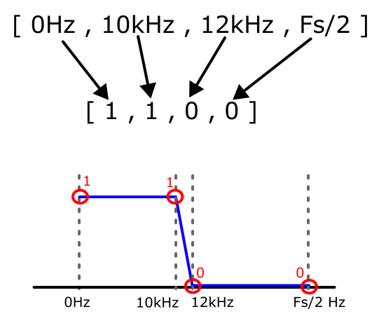
For example, suppose you wanted a low pass filter with a pass band starting at 0Hz (DC) then having a -3dB cutoff around 10kHz, then a transition band until the stop band at 12kHz. The bands parameter would look like:

[ 0, 10e3, 12e3, Fs/2 ]

Where Fs is your sampling frequency and Fs/2 is the max frequency of your filter before it starts repeating. For example if the sample rate is 100khz, then [ 0, 10e3, 12e3, 100e3/2 ] .

The desired parameter for this low pass filter would be:

[1, 1, 0, 0]

For example:

taps = signal.firls(numtaps, [0, 10e3, 12e3, 100e3/2], [1,1,0,0],fs=Fs)

Remez - Remez Exchange / Optimal / Parks-McClellan Exchange Method

The next method to generate filter coefficients is the Remez exchange method. These coefficients can be generated using the remez function:

taps = signal.remez(numberOfTaps, bands, desired, sampleFrequency )

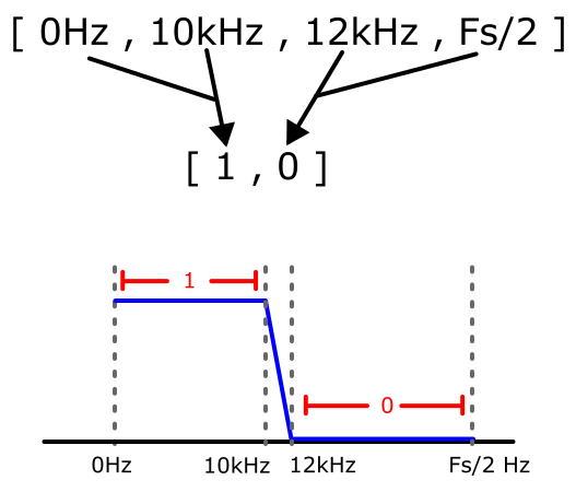
Which is very similar “format” as the firls but the desired parameter is defined a little differently. For example, suppose you wanted a low pass filter with a pass band starting at 0Hz (DC) then having a -3dB cutoff around 10kHz, then a transition band until the stop band at 12kHz. The bands parameter would look like:

[ 0, 10e3, 12e3, Fs/2 ]

The desired for this low pass filter would be:

[1, 0]

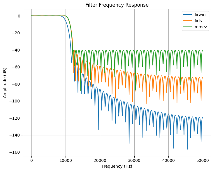
Plotting

Now with some methods to create our FIR filter coefficients, lets plot the responses using the freqz( ) function.

# Sample rate
Fs = 100e3

numtaps = 101

## Firwin

taps = signal.firwin(numtaps, cutoff=10e3, window='hann',fs=Fs)
f, h = signal.freqz(taps, [1], fs=Fs)

plt.figure(figsize=(10, 6))
plt.plot(f, 20 * np.log10(abs(h)), label="firwin")
plt.title('Filter Frequency Response')
plt.xlabel('Frequency (Hz)')
plt.ylabel('Amplitude (dB)')
plt.grid(True)
plt.show()

## Firls --------------------------------

taps = signal.firls(numtaps, [0, 10e3, 12e3, Fs/2], [1,1,0,0],fs=Fs)
f, h = signal.freqz(taps, [1], fs=Fs)

plt.plot(f, 20 * np.log10(abs(h)), label="firls")
plt.title('Filter Frequency Response')
plt.xlabel('Frequency (Hz)')
plt.ylabel('Amplitude (dB)')
plt.grid(True)
plt.legend()
plt.show()

## Remez --------------------------------

taps = signal.remez(numtaps, [0, 10e3, 12e3, Fs/2], [1, 0], fs=Fs)
f, h = signal.freqz(taps, [1], fs=Fs)

plt.plot(f, 20 * np.log10(abs(h)), label="remez")
plt.title('Filter Frequency Response')
plt.xlabel('Frequency (Hz)')
plt.ylabel('Amplitude (dB)')
plt.grid(True)
plt.legend()
plt.show()

Filtering a Signal

“Normal” Filtering

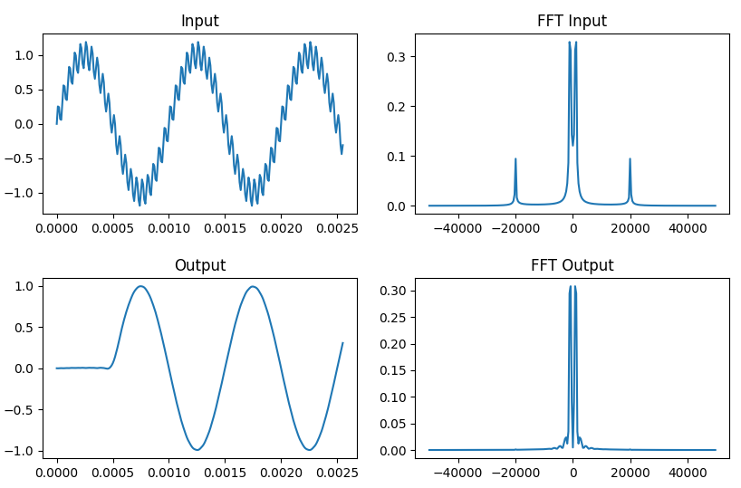
Now that we have a simple way to generate our filter coefficients, lets filter out a high frequency tone from our main signal. First we will create a signal with a tone at 1kHz and another tone at 20kHz.

# Number of sample points
N = int(2**8)

# Sample rate
Fs = 100e3
Ts = 1/Fs
sample = np.linspace(0.0,N*Ts, N, endpoint=False)

# Generate input signal with 1kHz and 20kHz tones
f1 = 1e3
f2 = 20e3
sig_in = 1*np.sin(f1*2.0*np.pi*sample) + 0.2*np.sin(f2*2.0*np.pi*sample)

Next we will create our low pass filter using the remez( ) function and then use lfilter( ) function to our sig_in signal to remove the 20kHz tone.

# Generate low pass filter coefficients
numtaps = 101
taps = signal.remez(numtaps, [0, 10e3, 12e3, Fs/2], [1, 0], fs=Fs)

# Filter input signal with lowpass filter
# Filtering out the 20kHz tone
sig_out = signal.lfilter(taps, [1], sig_in)

Putting this all together and plotting the results:

# Number of sample points
N = int(2**8)

# Sample rate
Fs = 100e3
Ts = 1/Fs
sample = np.linspace(0.0,N*Ts, N, endpoint=False)

# Generate input signal with 1kHz and 20kHz tones
f1 = 1e3
f2 = 20e3
sig_in = 1*np.sin(f1*2.0*np.pi*sample) + 0.2*np.sin(f2*2.0*np.pi*sample)

# Generate low pass filter coefficients
numtaps = 101
taps = signal.remez(numtaps, [0, 10e3, 12e3, Fs/2], [1, 0], fs=Fs)

# Filter input signal with lowpass filter
# Filtering out the 20kHz tone
sig_out = signal.lfilter(taps, [1], sig_in)


# Plot input signal in time
plt.figure()
plt.subplot(2,2,1)
plt.plot(sample, sig_in)
plt.title("Input")

# Plot output signal in time
plt.subplot(2,2,3)
plt.plot(sample, sig_out)
plt.title("Output")

# Plot input signal in frequency
yf = fftshift(fft(sig_in) * 1/N)
xf = fftshift(fftfreq(N, Ts))
plt.subplot(2,2,2)
plt.plot(xf, np.abs(yf))
plt.title("FFT Input")

# Plot input signal in frequency
yf = fftshift(fft(sig_out) * 1/N)
xf = fftshift(fftfreq(N, Ts))
plt.subplot(2,2,4)
plt.plot(xf, np.abs(yf))
plt.title("FFT Output")

Sample-By-Sample Filtering

In the previous section, we used lfilter() to process the entire sig_in signal at once. However, some applications, like real-time control systems with PID loops, require filtering samples one at a time.

To process samples individually while maintaining the filter's continuity, you need:

1. A for loop to iterate through each sample in sig_in.

2. A state variable (initialized as zeros) to store the filter’s internal delay registers.

3. An output array to store each processed sample.

The logic works as follows: by default, lfilter() resets its internal state to zero every time it is called. To prevent this, you must capture the final state (the "zi" output) from the current call and pass it back as the initial state (the "zi" input) for the next sample. At each iteration, you store the resulting filtered sample into your output array.

# Generate low pass filter coefficients
numtaps = 101
taps = signal.remez(numtaps, [0, 10e3, 12e3, Fs/2], [1, 0], fs=Fs)

# Create an all zero filter state array (ie the filter has just started up)
filterState = np.zeros(numtaps-1)

# Create an all zero output array to hold filtered signal
sig_out = np.zeros(N)

# Increment through each sample in the sig_in signal
for i in range(N):
    # Add the next sample into the FIR filter and calculate the output
    # Also save the filter state for the next loop itteration
    out, filterState = signal.lfilter(taps, [1], [sig_in[i]], zi=filterState)
    sig_out[i] = out[0]

Putting this all together and plotting the results:

import numpy as np
import matplotlib.pyplot as plt
from scipy.fft import fft, fftfreq, fftshift
from scipy import signal

# Number of sample points
N = int(2**8)

# Sample rate
Fs = 100e3
Ts = 1/Fs
sample = np.linspace(0.0,N*Ts, N, endpoint=False)

# Generate input signal with 1kHz and 20kHz tones
f1 = 1e3
f2 = 20e3
sig_in = 1*np.sin(f1*2.0*np.pi*sample) + 0.2*np.sin(f2*2.0*np.pi*sample)

# Generate low pass filter coefficients
numtaps = 101
taps = signal.remez(numtaps, [0, 10e3, 12e3, Fs/2], [1, 0], fs=Fs)

# Create an all zero filter state array (ie the filter has just started up)
filterState = np.zeros(numtaps-1)

# Create an all zero output array to hold filtered signal
sig_out = np.zeros(N)

# Increment through each sample in the sig_in signal
for i in range(N):
    # Add the next sample into the FIR filter and calculate the output
    # Also save the filter state for the next loop itteration
    out, filterState = signal.lfilter(taps, [1], [sig_in[i]], zi=filterState)
    sig_out[i] = out[0]



# Plot input signal in time
plt.figure()
plt.subplot(2,2,1)
plt.plot(sample, sig_in)
plt.title("Input")

# Plot output signal in time
plt.subplot(2,2,3)
plt.plot(sample, sig_out)
plt.title("Output")

# Plot input signal in frequency
yf = fftshift(fft(sig_in) * 1/N)
xf = fftshift(fftfreq(N, Ts))
plt.subplot(2,2,2)
plt.plot(xf, np.abs(yf))
plt.title("FFT Input")

# Plot input signal in frequency
yf = fftshift(fft(sig_out) * 1/N)
xf = fftshift(fftfreq(N, Ts))
plt.subplot(2,2,4)
plt.plot(xf, np.abs(yf))
plt.title("FFT Output")

Block-By-Block Filtering

This approach follows the same principle as sample-by-sample filtering, but instead, we process blocks of data and combine them into a single continuous output. This method is similar to using an ADC with DMA (Direct Memory Access): while the DMA fills one buffer, the processor handles the previously captured block. Once the DMA buffer is full, the processor begins processing that data while the next block of new data starts filling the DMA again.

# Number of sample points
N = int(2**8)

# Sample rate
Fs = 100e3
Ts = 1/Fs
sample = np.linspace(0.0,N*Ts, N, endpoint=False)

# Generate input signal with 1kHz and 20kHz tones
f1 = 1e3
f2 = 20e3
sig_in = 1*np.sin(f1*2.0*np.pi*sample) + 0.2*np.sin(f2*2.0*np.pi*sample)

# Break our input signal into smaller chunks
sig_in1 = sig_in[:85:]
sig_in2 = sig_in[85:170:]
sig_in3 = sig_in[170::]


# Generate low pass filter coefficients
numtaps = 101
taps = signal.remez(numtaps, [0, 10e3, 12e3, Fs/2], [1, 0], fs=Fs)

# Create an all zero filter state array (ie the filter has just started up)
filterState = np.zeros(numtaps-1)

## Process Data in Blocks ---------------

# Block 1
out, filterState = signal.lfilter(taps, [1], sig_in1, zi=filterState)
sig_out = out

## "DELAY" to revieve another block of data
    
# Block 2
out, filterState = signal.lfilter(taps, [1], sig_in2, zi=filterState)
sig_out = np.append(sig_out, out)   

## "DELAY" to revieve another block of data

# Block 3
out, filterState = signal.lfilter(taps, [1], sig_in3, zi=filterState)
sig_out = np.append(sig_out, out) 


# The above is a pretty basic example of this processing blocks. In reality
# you probably want a for loop that cycles through each block 


# Plot input signal in time
plt.figure()
plt.subplot(2,2,1)
plt.plot(sample, sig_in)
plt.title("Input")

# Plot output signal in time
plt.subplot(2,2,3)
plt.plot(sample, sig_out)
plt.title("Output")

# Plot input signal in frequency
yf = fftshift(fft(sig_in) * 1/N)
xf = fftshift(fftfreq(N, Ts))
plt.subplot(2,2,2)
plt.plot(xf, np.abs(yf))
plt.title("FFT Input")

# Plot input signal in frequency
yf = fftshift(fft(sig_out) * 1/N)
xf = fftshift(fftfreq(N, Ts))
plt.subplot(2,2,4)
plt.plot(xf, np.abs(yf))
plt.title("FFT Output")